|

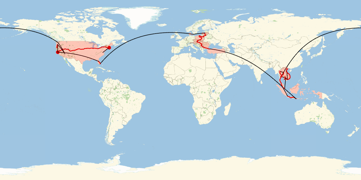
The image above, which describes my and Katie's 2015 travels, is built with the following Mathematica code:
map = GeoGraphics[Join[visitedCountries, pathsLatLong, annotations],
  GeoRange -> "World", GeoBackground -> GeoStyling["StreetMapNoLabels"], ImageSize -> 1200]
The GeoGraphics function is an exciting new capability of Mathematica
10 that can (among other things) project geography-related polygons and paths (expressed in latitude and longitude) on
a variety of global and regional projections. The default projection is equirectangular, which is fine for a first try. Let's shade in light red the countries we
visited as follows:
countryList = {"UnitedStates", "Thailand", "Malaysia", "Singapore",
   "Cambodia", "Vietnam", "Laos", "Indonesia", "Turkey", "Bulgaria",
   "Serbia", "Romania", "Hungary", "Slovakia", "CzechRepublic",
   "Austria", "Poland", "Lithuania", "Latvia", "Denmark"};
visitedCountries = {FaceForm[Red], Polygon[Entity["Country", #]]} & /@
    countryList;
We then accumulate air and ground paths of travel, which is more complex. First, let's input the cities we visited in order from October 31, 2014 to November 19, 2015:
cityList = {"Boston", "Richmond", "Boston", "Chicago", "Denver",
   "San Francisco", "Portland", "Medford", "Portland", "Las Vegas",
   "Seattle", "Bangkok", "Penang", "Kuala Lumpur", "Singapore",
   "Phnom Penh", "Sihanoukville", "Phnom Penh", "Siem Reap",
   "Phnom Penh", "Ho Chi Minh City", "Vung Tau", "Ho Chi Minh City",
   "Hanoi", "Cat Ba", "Hanoi", "Da Nang", "Hoi An", "Da Nang",
   "Nha Trang", "Ho Chi Minh City", "Bangkok", "Vientiane",
   "Udon Thani", "Chiang Mai", "Bangkok", "Pattaya", "Bangkok",
   "Hua Hin", "Kuala Lumpur", "Singapore", "Denpasar", "Ubud",
   "Denpasar", "Surabaya", "Yogyakarta", "Jakarta", "Kuala Lumpur",
   "Istanbul", "Plovdiv", "Sofia", "Belgrade", "Timisoara",
   "Budapest", "Bratislava", "Vienna", "Bratislava", "Brno", "Krakow",
    "Warsaw", "Gdansk", "Bialystok", "Vilnius", "Riga", "Copenhagen",
   "Fort Lauderdale", "The Villages", "Orlando", "San Francisco"};
Second, let's iterate through pairs of cities and look for driving directions (which I downloaded from Google Maps in KML format for the cases in which we took a bus or a train between cities). If a
driving directions file isn't present (i.e., when we flew), the code uses GeoPath to create a great-circle segment, pulls out the constitutive
Line components using Position, and styles the path in black. If
the directions file does exist, the code pulls out the appropriate path and styles it in red:
projectionsLocation = SetDirectory["C:/Users/John/Dropbox/Projections"];
pathsLatLong = Flatten[Rest[Reap[Do[
      fileName =
       Select[FileNames["Directions from " ~~ cityList[[i]] ~~ "*.kml", {projectionsLocation}],
        StringContainsQ[#, cityList[[i + 1]]] &];
      {route, coordinates, style} = If[fileName == {},
        {"air",
         Reverse /@ First@Extract[#, Replace[Position[#, Line], 0 -> 1, -1]] &@
          GeoGraphics[GeoPath[CityData[cityList[[#]], "Coordinates"] & /@ {i, i + 1}], GeoRange -> "World"],
         {Black, Thickness[0.0015], JoinForm["Round"]}},
        {"ground",
         Extract[#, Replace[Position[#, Line], 0 -> 1, -1]][[1, 1, All, 1 ;; 2]] &@
          Import[First@fileName, {"Data", 1, "Geometry"}],
         {Darker[Red, 0.15], Thickness[0.002], JoinForm["Round"]}}
        ];
      Sow[Append[style, Line[GeoPosition[coordinates]]], "tag"],
      {i, 1, Length[cityList] - 1}], "tag"]], 2];
I had to add the "tag" in Sow because there appears to be a Sow somewhere in the Replace function that was sending back unneeded data to my Reap.
We add the highlights at our beginning and end points as follows:
annotations = {Darker[Red, 0.15], PointSize[0.01], Point[GeoPosition[CityData[#, "Coordinates"]]]} & /@ {"Boston", "San Francisco"};
The GeoGraphics function can then be used as shown above to create the composite image.
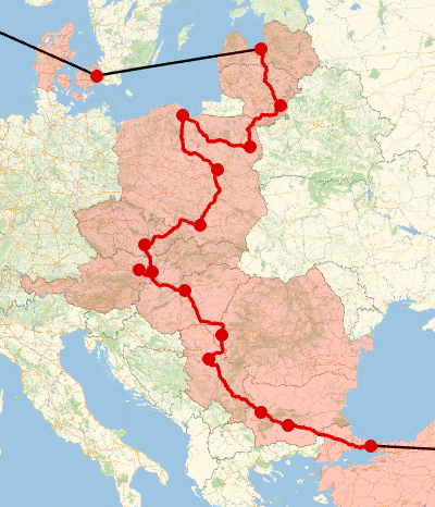
It's also possible to show just a portion of the trip. For example, the following
code adds red circles at each visited city in Europe (with Istanbul, which Mathematica considers an Asian city, added manually):
visitedCities = {Darker[Red, 0.15], PointSize[0.03], Point[GeoPosition[CityData[#, "Coordinates"]]]} & /@
   Prepend[Quiet@Select[cityList, CountryData[CityData[#, "Country"], "Continent"] ===
        EntityClass["Country", "Europe"] &], "Istanbul"];
GeoGraphics[
 Join[pathsLatLong /. Thickness[x_] -> Thickness[4 x],
  visitedCountries, visitedCities],
 GeoRange -> {{39, 58.5}, {10, 32}},
 GeoBackground -> GeoStyling["StreetMapNoLabels"], GeoZoomLevel -> 6,
 GeoRangePadding -> Full, ImageSize -> 400]
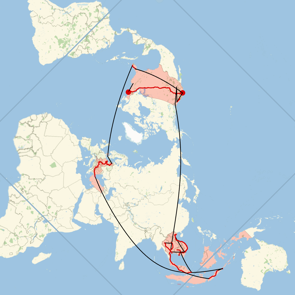
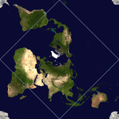
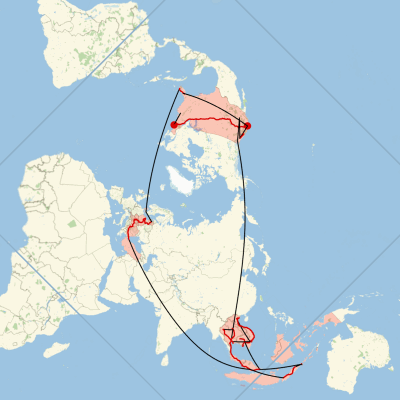
OK, that's neat enough, but I was interested in showing the path as closed to emphasize the round-the-world nature of our trip.
I settled on the Peirce quincuncial projection because it's centered on the North Pole and because it has the neat property that
the equator is transformed into a diamond:
However, this projection isn't (yet) built into Mathematica, so we need to do a little more work. I found the following code online
that was contributed by Stack Exchange
member J.M. (not me!):
SetAttributes[cnhalf, Listable];
cnhalf[z_?NumericQ] := Block[{nz = N[z], k, zs}, k = Max[0, Ceiling[Log2[4 Abs[nz]]]];
  zs = (nz 2^-k)^2;
  Nest[With[{cs = #^2}, -(((cs + 2) cs - 1)/((cs - 2) cs - 1))] &, (1 - zs/4 (1 + zs/30 (1 + zs/8)))/(1 + zs/4 (1 - zs/30 (1 - zs/8))), k]]
to be used in conjunction with With[{w = cnhalf[#[[1]] + I #[[2]]]}, {Arg[w], 2 ArcCot[Abs[w]]}] & inside
the ImageTransformation function. That person also supplied a function to transform equirectangular coordinates:
Through[{Re, Im}[InverseJacobiCN[Cot[φ°/2 + π/4] Exp[I θ°], 1/2]]]. Cool! So
let's get an equirectangular projection again with red-shaded countries and image-transform it:
mapSize = N[EllipticK[1/2], 20];
background = ImageTransformation[
   GeoGraphics[{FaceForm[Red], Polygon[Entity["Country", #]]} & /@ countryList, GeoRange -> "World", ImageSize -> 2400,
    GeoBackground -> GeoStyling["StreetMapNoLabels"], GeoZoomLevel -> 3],
   With[{w = cnhalf[#[[1]] + I #[[2]]]}, {Arg[w], 2 ArcCot[Abs[w]]}] &,
   DataRange -> {{-π, π}, {0, π}}, Padding -> 1.,
   PlotRange -> {{0, 2 mapSize}, {-mapSize, mapSize}}];
Now let's assemble our paths as before, but this time we'll want them in (longitude, latitude) (i.e., (x, y)) coordinate form instead of (latitude, longitude)
form because we'll be using Graphics instead of GeoGraphics:
pathsLongLat = Flatten[Rest[Reap[Do[
      fileName = Select[FileNames["Directions from " ~~ cityList[[i]] ~~ "*.kml", {projectionsLocation}], StringContainsQ[#, cityList[[i + 1]]] &];
      {route, coordinates, style} = If[fileName == {},
        {"air",
         First@Extract[#, Replace[Position[#, Line], 0 -> 1, -1]] &@
          GeoGraphics[GeoPath[CityData[cityList[[#]], "Coordinates"] & /@ {i, i + 1}], GeoRange -> "World"],
         {Black, Thickness[0.002], JoinForm["Round"]}},
        {"ground",
         Extract[#, Replace[Position[#, Line], 0 -> 1, -1]][[1, 1, All, 2 ;; 1 ;; -1]] &@
          Import[First@fileName, {"Data", 1, "Geometry"}], {Darker[Red, 0.15], Thickness[0.0026], JoinForm["Round"]}}
        ];
      Sow[Append[style, Line[coordinates]], "tag"],
      {i, 1, Length[cityList] - 1}], "tag"]], 2];
The image transformation leaves a line on the right, which we can cover using a sea-colored line:
cleanup =
  Graphics[{RGBColor[{158, 197, 225}/255], Thickness[0.005],
    Line[#] & /@ {{{mapSize, 0}, {1.14 mapSize, 0}}, {{1.19 mapSize,
        0}, {2 mapSize, 0}}}}, ImagePadding -> None,
   PlotRangePadding -> None];
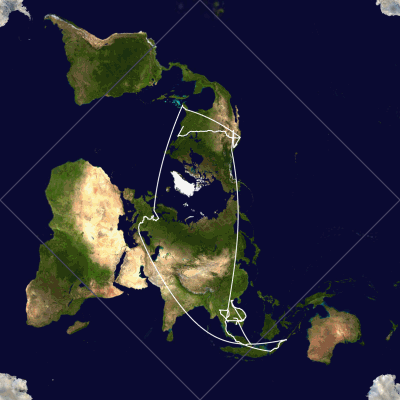
Finally, we add a darker blue equator, highlight beginning and end points, transform all the coordinates from equirectangular to Peirce quincuncial, assemble the composite image, and crop out latitudes we didn't visit:
ImageCompose[background,
  Show[cleanup,
   Graphics[
    Join[{EdgeForm[{Darker[RGBColor[{158, 197, 225}/255], 0.1], Thickness[0.003]}], FaceForm[None], Polygon[{{0, 0}, {90, 0}, {180, 0}, {270, 0}}]},
     {Darker[Red, 0.15], PointSize[0.015],
     Point[Reverse[CityData[#, "Coordinates"]]]} & /@ {"Boston", "San Francisco"},
     pathsLongLat] /.
      {\[Theta]_?NumericQ, \[CurlyPhi]_?NumericQ} :>
       Through[{Re, Im}[InverseJacobiCN[Cot[φ°/2 + π/4] Exp[I θ°], 1/2]]],
    ImagePadding -> None, PlotRangePadding -> None]]];
map = ImageCrop[#, 0.85 First@ImageDimensions[#]] &@%
|