Generalized Hooke’s Law is a compact and powerful equation describing any linear elastic* deformation of any isotropic** material:
$$\varepsilon_{ij}=\frac{1+\nu}{E}\sigma_{ij}-\frac{\nu}{E}\sigma_{kk}\delta_{ij};$$
where \(\varepsilon\) is the strain, \(\nu\) is Poisson’s ratio, \(E\) is Young’s modulus, \(\sigma\) is the stress, \(\delta\) is the Kronecker delta (I’ll explain all this notation below), and the subscripts \(i\), \(j\) and \(k\), also called the indices, can range from 1 to 3, corresponding to three orthogonal directions, such as \(x\), \(y\), and \(z\):
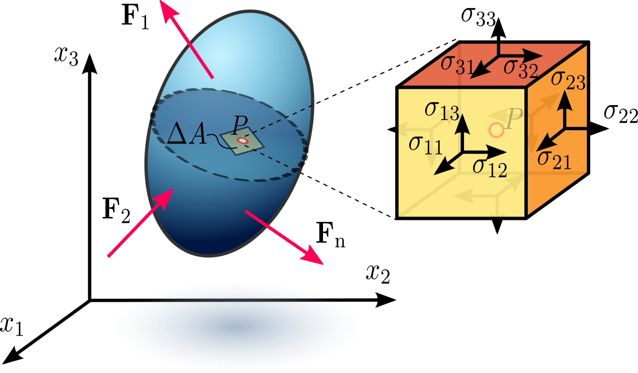
A 3D body can be subjected to a variety of surface and body forces that result in a complex state of normal and shear stresses and, in turn, normal and shear strains. ***REDRAW WITH FUSION TO INCLUDE MAYBE A BODY FORCE, A NORMAL FORCE, ETC., MAYBE STRESS FROM CONSTRAINED THERMAL EXPANSION***
*Linear elastic materials deform twice as much when you double the load, and all deformation is recovered when the load is removed. All stable materials are approximately linearly elastic for suitably small deformations.
**Isotropic materials look the same from all directions. Examples? Amorphous ceramics such as window glass have no strongly preferred direction and are thus considered isotropic. Metals are generally polycrystalline, and their grain orientation in bulk form is often sufficiently random that any directional influence is negligible, so they can also often be considered isotropic. What materials aren’t isotropic? The single-crystal silicon used in wafers for integrated circuit manufacturing, for example. Single-crystal turbine blades and metal whiskers. Thin polycrystalline films or strongly deformed bulk metals in which the grains have a preferred direction. Composites, in which certain stress-bearing materials are often oriented in specific directions. You get the idea.
Remarkably, we can derive the broad relation above using only two assumptions:
All stable materials stretch when pulled and contract when pushed. To characterize this effect, let’s assume that for a long, thin object (termed a rod or a bar) being pulled or pushed down its length, the linear elastic equation \(\sigma=E\varepsilon\) applies, where \(\sigma\) is the uniaxial stress, or the axial force over the cross-sectional area and \(\varepsilon\) is the uniaxial strain, or the axial deformation over the length. This is simple Hooke’s Law. It also serves as a definition of Young’s elastic modulus \(E\).
(Elastic moduli are generally useful because we wish to understand how a solid pulls or pushes back in response to suitably small forces. At large forces, the predominant mechanism or the geometry may change; this the realm of nonlinear elasticity. Alternatively, the sample may not recover; this is the realm of plasticity. This note assumes small forces, deformations, stresses, and strains.)
The lateral dimensions may also change. We define a single additional material property, Poisson’s ratio \(\nu\), as the strain ratio of the lateral contraction to the longitudinal expansion: \(\nu=-\varepsilon_2/\varepsilon_1=-\varepsilon_3/\varepsilon_1\). Poisson’s ratio is usually positive; that is, most materials tend to contract laterally when you stretch them:

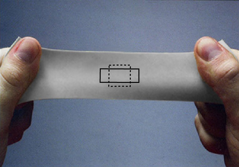
Axial elongation and lateral contraction from a tensile load. (Image based on a photograph by Nielson Fitness.)
These two concepts (and two material properties) alone are enough to cover all linearly elastic stress and strain states in any isotropic material and to derive generalized Hooke’s Law. And the benefits arguably outweigh the work to get there. With a little manipulation, for example, generalized Hooke’s Law provides the definitions of other widely used moduli (the shear modulus, the bulk modulus, and the biaxial and plane strain moduli, for example). The relations between these moduli and Young’s modulus are frequently noted in reference materials but less frequently derived; knowledge of generalized Hooke’s Law makes their derivation easy. But more broadly, generalized Hooke’s Law allows us to explore the deformation of geometries other than rods and bars—wide beams, plates, thin films, seismic waves, and objects under various types of constraints, for example. And thermal expansion is easily incorporated. All these scenarios are discussed below.
The details
To derive generalized Hooke’s Law, we need to move beyond the uniaxial nature of simple Hooke’s Law \(\sigma=E\varepsilon\) and look at how stresses and strains are defined and are coupled in 3D. We’ll first address 3D stress.
Understanding normal and shear stresses in 3D
Consider two distinct ways to apply a surface force on an object: perpendicular (or normal) to the surface (to produce a normal stress) or parallel with the surface (to produce a shear stress):
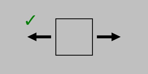
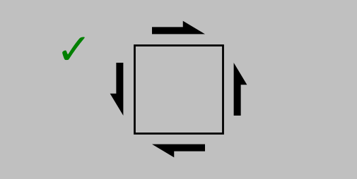
Elasticity involves static conditions only; all forces in every direction—and even around every axis—must balance. (Even the simple state of static equilibrium leaves us enough to worry about.) (Created in Python using this code.)
But in both cases, to prevent the object from accelerating away or beginning to spin, we need to add some additional forces to describe the complete stress state. And although we started with the example of a surface, we can think of these stress states appearing anywhere in a body; thus, the 2D square shown above represents a very small region (a differential element) in any 3D orientation and in any location.
The combinations of possible stresses in 3D are distinguished by an index \(i\) for the direction of the force and an index \(j\) for the direction perpendicular to the surface; thus, \(\sigma_{12}\) represents the stress from a force in the 1 direction pulling on a surface oriented in the 2 direction. Static equilibrium conditions let us drop pairs of minus signs (thus, \(\sigma_{(-1)(-1)}=\sigma_{11}\), for example, as in the correctly drawn normal stress example above). They also require \(\sigma_{ij}=\sigma_{ji}\) to prevent rotation. (Try drawing the schematics for \(\sigma_{ij}\) and \(\sigma_{ji}\), including all the surface forces necessary to prevent acceleration. You’ll find that the resulting schematics are identical.)
The resulting set of 3D stresses for \(i, j =1\mbox{–}3\) is a tensor, meaning that it couples algebraic objects (here, corresponding to forces and areas). And because those algebraic objects are each vectors themselves (specifically, a force vector and a surface normal vector), or first-order tensors, the stress tensor that couples them is in turn specifically a second-order tensor, which can be written in matrix form:
$$\boldsymbol{\sigma}=\sigma_{ij}=\left[\begin{array}{c}
\sigma_{11} & \sigma_{12} & \sigma_{13}\\
& \sigma_{22} & \sigma_{23}\\
\mbox{sym.}& &\sigma_{33}\\
\end{array}\right].
$$
The numbers of rows and columns equal the dimensionality of the problem, which is 3. (For clarity, vectors and higher-order tensors are written in boldface in this note.)
Moving on to 3D strain…
Understanding normal and shear strains in 3D
First up is the case of normal strain, quantified by the relative elongation of a line pointing in a certain direction. Note especially the movement and direction of the displacement (let’s call it \(\color{green}{\boldsymbol{u}}\)) relative to the orientation and length of the original vector \(\color{blue}{\boldsymbol{x}}\).
A vector \(\color{blue}{\boldsymbol{x}}\) undergoing normal strain. Below, the initial length of the vector, \(\color{blue}{x_1}\), and the displacement \(\color{green}{u_1}\) of its tip relative to its tail.
Normal strains tend to change differential element side lengths. We could handle this case with a simple ratio of vector magnitudes if we wished. (That is, we could divide \(|\color{green}{\boldsymbol{u}}|\) by \(|\color{blue}{\boldsymbol{x}}|\), and this scheme works regardless of whether we fix any edge or point of the differential element.)
Things become more ambiguous, however, when we consider shear strains, which instead tend to change element corner angles:

Shear strain: two orthogonal original vectors and the displacements of their tips relative to their tails. The results now differ depending on which edge or point we consider fixed. But any discrepancy can be eliminated if we consider the average relative deformation of both vectors in the 1 and 2 directions. (Another useful definition is the engineering shear stress \(\gamma\), which is simply the reduction in the top-right or bottom-left angle.)
Any scheme of simply taking the ratio of two vectors now runs into a problem: which initial vector should we pick—the one pointing in the 1 direction or the one pointing in the 2 direction? This problem is resolved by defining the tensorial shear strain as XXX
$$\varepsilon_{ij}=\frac{1}{2}\left(\frac{\partial \color{green}{u_i}}{\partial \color{blue}{x_j}}+\frac{\partial \color{green}{u_j}}{\partial \color{blue}{x_i}}\right),$$
which works because the two scenarios are averaged together. The connection with angular changes comes about because when \(\color{green}{\boldsymbol{u}}\) is perpendicular to \(\color{blue}{\boldsymbol{x}}\), \(|\color{green}{\boldsymbol{u}}|/|\color{blue}{\boldsymbol{x}}|\) equals the tangent of the included angle, which for small \(\color{green}{\boldsymbol{u}}\) is approximately equal to the angle itself (in radians).
Even better, this definition works for normal strains too, where \(i=j\), because
$$\varepsilon_{11}=\frac{1}{2}\left(\partial \color{green}{u_1}/\partial\color{blue}{x_1}+\partial \color{green}{u_1}/\partial\color{blue}{x_1}\right)=\partial \color{green}{u_1}/\partial\color{blue}{x_1},$$
for direction 1, for example, so we have a definition we can apply to both scenarios. Note that the additive tensorial strain definition also provides symmetry: \(\varepsilon_{ij}=\varepsilon_{ji}\). So both the stress and strain tensors are symmetric; the latter is
$$\boldsymbol{\varepsilon}=\varepsilon_{ij}=\left[\begin{array}{c}
\varepsilon_{11} & \varepsilon_{12} & \varepsilon_{11}\\
& \varepsilon_{22} & \varepsilon_{23}\\
\mbox{sym.}& &\varepsilon_{31}\\
\end{array}\right].
$$
(The engineering shear strain \(\gamma\) is also widely used; it’s defined simply as the reduction in a right angle of a differential element as shown above. The engineering shear strain is twice the tensorial shear strain.)
We can now establish the equations that comprise generalized Hooke’s Law.
Defining and assembling the constitutive equations
In fact, generalized Hooke’s Law ultimately describes six (!) separate deformation situations with one equation. The first three situations couple normal stresses with normal strains. For a general 3D chunk of isotropic material, in any direction \(i\), we can expect longitudinal deformation from a normal stress oriented in the \(i\) direction and lateral (Poisson) deformation from normal stresses oriented in the other two directions—the \(j\) and \(k\) directions. According to the definitions of Young’s modulus and Poisson’s ratio above, we can express the normal strains as
$$\varepsilon_{11}=\frac{1}{E}\sigma_{11}-\frac{\nu }{E}\sigma_{22}-\frac{\nu }{E}\sigma_{33};$$
$$\varepsilon_{22}=\frac{1}{E}\sigma_{22}-\frac{\nu }{E}\sigma_{11}-\frac{\nu }{E}\sigma_{33};$$
$$\varepsilon_{33}=\frac{1}{E}\sigma_{33}-\frac{\nu }{E}\sigma_{11}-\frac{\nu }{E}\sigma_{22}.$$
That is, in the 3D framework of generalized Hooke’s Law, any positive/negative normal stress in any direction causes elongational/contractile strain in that direction (as mediated by Young’s modulus) and lateral strain in the other directions (as mediated by Young’s modulus and Poisson’s ratio).
The second three situations couple shear stresses with shear strains and require some geometrical craftiness to apply our two primary assumptions. Consider the deformation state shown below on the left for pure shear. We’ll want to transform this stress state into one involving a normal stress so that we can apply our initial assumptions involving Young’s modulus and Poisson’s ratio. An equivalent stress state is shown on the right that involves only normal stresses in an orientation (\(1^\prime\)-\(2^\prime\)) that’s tilted by 45° from the original one:
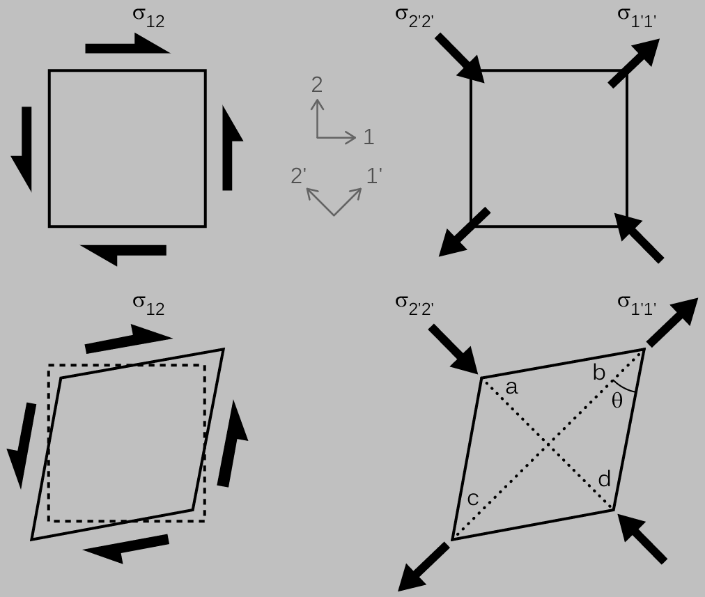
Caption ***FIX ARROWS AND MAKE SIZES CONSISTENT WITH THE OTHER FIGURES; SHIFT COORDINATE SYSTEMS TO THEIR RESPECTIVE SIDES***
From symmetry, we could hypothesize that the magnitude of \(\sigma_{1^\prime 1^\prime}\) should equal that of \(\sigma_{2^\prime 2^\prime}\). Although it’s outside the scope of this note, a Mohr’s circle analysis would confirm this hypothesis and also show that \(\sigma_{12}\), \(\sigma_{1^\prime 1^\prime}\), and \(\sigma_{2^\prime 2^\prime}\) all have the same magnitude.
Along line bc, based on the equations linking normal stress and normal strain, we expect an elongational strain from the tensile stress \(\sigma_{1^\prime 1^\prime}\) and another one (a Poisson-mediated one) from the compressive strain \(\sigma_{2^\prime 2^\prime}\) of the same magnitude:
$$\varepsilon_{1^\prime 1^\prime}=\frac{1+\nu}{E}\sigma_{1^\prime 1^\prime}.$$
For line ad, we expect an contractile strain from \(\sigma_{2^\prime 2^\prime}\) and another one (a Poisson-mediated one) from \(\sigma_{1^\prime 1^\prime}\):
$$\varepsilon_{2^\prime 2^\prime}=-\frac{1+\nu}{E}\sigma_{1^\prime 1^\prime}=-\varepsilon_{1^\prime 1^\prime}.$$
Applying trigonometry to the diagram above, we find that the angle \(\theta\), which was initially 45° or \(\pi/4\) (satisfying \(\arctan\left(\frac{|ad|/2}{|bc|/2}\right)=\arctan(1)\) because lines bc and ad were of equal length) now satisfies
$$\theta=\arctan\left(\frac{(1+\varepsilon_{2^\prime 2^\prime})/2}{(1+\varepsilon_{1^\prime 1^\prime})/2}\right)=\arctan\left(\frac{1-\varepsilon_{1^\prime 1^\prime}}{1+\varepsilon_{1^\prime 1^\prime}}\right).$$
Multiplication by \(\frac{1-\varepsilon_{1^\prime 1^\prime}}{1-\varepsilon_{1^\prime 1^\prime}}\) within the arctangent argument and dropping any \(\varepsilon^2\) terms as neglibly small gives
$$\theta=\arctan(1-2\varepsilon_{1^\prime 1^\prime}). $$
This looks like the arctangent of 1 minus a small value—a great candidate for Taylor series expansion. (I try to never miss a chance to apply a Taylor series expansion.) Specifically, a Taylor series restates any function \(f\) evaluated at \(x_0+\delta x\) as
$$f(x_0+\delta x)=f(x_0)+f^\prime (x_0)\delta x+\frac{1}{2!}f^{\prime\prime} (x_0)(\delta x)^2+\frac{1}{3!}f^{\prime\prime\prime} (x_0)(\delta x)^3\cdots.$$
where the prime notation indicates a derivative. This expansion is useful when we know \(f\) and its derivatives at \(x_0\) but not \(f(x_0+\delta x\).
(Expressed in words, this series of terms means simply that near \(x_0\), any smooth function takes a value similar to that at \(x_0\) but with a slope-based linear correction for the distance between \(x_0\) and \(x_0+\delta x\), and we might add a slight correction for the quadratic curvature of \(f\), and maybe the tiniest correction for any additional cubic character, and so on.)
The smaller \(\delta x\) is, the fewer terms we need for a good approximation. In this case, let’s evaluate \(\arctan(1-2\varepsilon_{1^\prime 1^\prime})\) with just two terms:
$$\arctan(1-2\varepsilon_{1^\prime 1^\prime})\approx\arctan(1)+\frac{1}{1+1^2}(-2\varepsilon_{1^\prime 1^\prime})=\frac{\pi}{4}-\varepsilon_{1^\prime 1^\prime}$$
because the derivative of \(\arctan(x)\) is \(1/(1+x^2)\). Thus, the decrease in the 45° angle, corresponding to the tensorial shear stress and half the engineering shear stress, is \(\varepsilon_{1^\prime 1^\prime}=(1+\nu)\sigma_{1^\prime 1^\prime}/E=(1+\nu)\sigma_{12}/E\).
Since this relation can be applied in the 1-2, 1-3, and 2-3 directions, we have three new equations:
$$\varepsilon_{12}=\frac{1+\nu}{E}\sigma_{12}; $$
$$\varepsilon_{13}=\frac{1+\nu}{E}\sigma_{13}; $$
$$\varepsilon_{23}=\frac{1+\nu}{E}\sigma_{23}. $$
Generalized Hooke’s Law, then, needs to encompass all of this information (six equations coupling normal and shear stresses with normal and shear strains in 3D) in a single equation, and it does so with the help of two notational tools:
The repetition of a dummy index within a certain term implies summation over the range of indices; i.e., \(\sigma_{kk}=\sigma_{11}+\sigma_{22}+\sigma_{33}\), for example. (This is called Einstein summation.)
The Kronecker delta \(\delta_{ij}\) is 1 if \(i=j\) and 0 otherwise.
Thus, we can write
$$\varepsilon_{ij}=\frac{1+\nu}{E}\sigma_{ij}-\frac{\nu}{E}\sigma_{kk}\delta_{ij}.$$
Take a second to recognize how this equation simplifies in the normal strain case (when \(\delta_{ij}=1\)) and in the shear strain case (when \(\delta_{ij}=0\)) to obtain each of the six individual equations above.
Furthermore, these six equations can also be solved for strain instead of stress, giving
$$ \sigma_{ij}=\frac{E}{1+\nu}\varepsilon_{ij}+\frac{\nu E}{(1+\nu)(1-2\nu)}\varepsilon_{kk}\delta_{ij},$$
which we’ll also find useful.
Well, that wrapped up nicely, with no loose ends. Well…
Why aren’t shear strains dependent on normal stresses (or normal strains on shear stresses)?
In the above derivation, normal strains were linked to normal stresses and shear strains to shear stresses, but no cross coupling was discussed. Here’s why. If a normal stress were to cause a shear strain, for example, then we’d expect something like the state of loading and deformation shown below in (a), where the purple dot is used to mark the orientation of the differential element. We could always flip this picture upside down to obtain (b), of course. But since an isotropic material looks the same for all orientations, we should instead expect that the flipped material gives the same shear response as in (a), which is shown in (c). This paradox—the fact that (b) and (c) don’t match—leaves us to conclude that there cannot be any shear strain in this case.
Similar symmetry arguments, involving reflection and rotation, can be applied for various other circumstances and crystal structures to helpfully identify elastic coupling constants that must be zero. In fact, if we briefly drop the condition of isotropy, as assumed elsewhere in this note, a still broader framework applies: \(\boldsymbol{\sigma}=\boldsymbol{C}\boldsymbol{\varepsilon}\), where \(\boldsymbol{C}\) is a fourth-order (!) tensor, called the stiffness tensor, that couples the two second-order tensors of 3D stress and 3D strain. The dimensionality being 3, the fourth-order stiffness tensor has \(3^4=81\) components. Symmetry arguments can be used to show that most of the elements of \(\boldsymbol{C}\) are zero for isotropic materials. For example, \(C_{1112}=0\) because the normal stress \(\sigma_{11}\) is independent of the shear strain \(\varepsilon_{12}\), as shown above through reflection/mirror arguments. What about \(C_{1111}\), which couples the normal stress \(\sigma_{11}\) to the normal strain \(\sigma_{11}\)? What about \(C_{1122}\)? \(C_{2113}\)?
The benefits
It’s now straighforward to apply generalized Hooke’s Law
$$\varepsilon_{ij}=\frac{1+\nu}{E}\sigma_{ij}-\frac{\nu}{E}\sigma_{kk}\delta_{ij},$$
with the first application being the definition of various moduli.
1. Uniaxial stress states. This first example is mostly recapitulation with terms and concepts that are now familiar. In other words, we’ll now communicate as material scientists do. Consider the case of a rod or bar (by definition, a long, thin object) under uniaxial loading along the 1-axis and no other loading. For a long, thin structure, we can assume that any internal region is close enough to the stress-free sides that the lateral stresses \(\sigma_{22}\) and \(\sigma_{33}\) are always zero. Inserting these conditions into generalized Hooke’s Law, we obtain uniaxial (simple) Hooke’s Law along with the expected lateral strain associated with Poisson’s ratio:
$$\varepsilon_{11}=\frac{1}{E}\sigma_{11};$$
$$\varepsilon_{22}=\varepsilon_{33}=-\frac{\nu}{E}\sigma_{11}.$$
All shear strains are zero. These specific conditions serve to define Young’s modulus: \(E=\sigma_{11}/\varepsilon_{11}\).
2. Pure shear shear states. In the case of pure shear (\(\sigma_{12}\) nonzero, all other stresses zero), we obtain from generalized Hooke’s Law
$$\varepsilon_{12}=\frac{1+\nu}{E}\sigma_{12},$$
and all other strains are zero.
The shear modulus \(G\) is defined as the ratio of the shear stress \(\sigma_{ij}\) to the engineering shear strain \(\gamma_{ij}\); as noted earlier, \(\gamma_{ij}=2\varepsilon_{ij}\), so the shear modulus is defined under these conditions as
$$G=\frac{E}{2(1+\nu)}.$$
3. Hydrostatic pressure states. Let’s assume now that the stress state is hydrostatic (all shear stresses zero, normal stresses \(\sigma_{11}=\sigma_{22}=\sigma_{33}=-P\), where the positive number \(P\) is the pressure; this stress state is also called an equitriaxial compressive stress state). From generalized Hooke’s Law, the normal strain in any direction is then
$$\varepsilon=-\frac{1-2\nu}{E}P,$$
while all shear strains are found to be zero. The bulk modulus \(K\) is defined as the pressure required to obtain a certain normalized reduction in volume. (Put another way, the bulk modulus couples the hydrostatic stress to the negative volumetric strain.) It’s handy at this point to think of a cube with side length \(L\), so that the initial volume is \(L^3\) and the final volume is \([L(1+\varepsilon)]^3\). The reduction in volume, normalized to the volume, is then
$$-\frac{\Delta V}{V}=-[(1+\varepsilon)^3-1].$$
Hey, the term \((1+\varepsilon)^3\) looks like another outstanding candidate for Taylor series expansion since \(\varepsilon\) is small. The function \(f\) is the cubic function, and we find that
$$(1+\varepsilon)^3\approx 1+3(1)^2\varepsilon=1+3\varepsilon.$$
Thus, the bulk modulus is
$$K=\frac{P}{-\Delta V/V}=-\frac{P}{3\varepsilon}=\frac{E}{3(1-2\nu)}.$$
I wrote elsewhere about how important the shear and bulk moduli are in our understanding of real 3D materials, even though Young’s modulus gets predominant attention. The shear modulus governs how objects under stress change their shape, whereas the bulk modulus governs how these objects change their size. When we stretch an object uniaxially, a mishmash of these two states applies, which is somewhat unsatisfying conceptually—on the one hand. On the other hand, it’s relatively easy to mount a dogbone tensile sample into a uniaxial testing tool and experimentally obtain Young’s modulus and Poisson’s ratio. The best material handbooks will provide Young's modulus, the shear modulus, and Poisson's ratio, which is all you need to fully characterize an isotropic and linearly elastic material.
4. Plane strain states (which arise in constrained objects and in wide beams and plates, for example). Consider the case where the strain in a certain direction (the 3-direction, say) is constrained to be zero. This is called plane strain: all strains are confined to one plane (here, the 1–2 plane). How does this state arise? Perhaps our object is constrained in one direction by a much more rigid structure. One classic example is an object mounted between two unyielding walls:
(Graphic)
We also see a plane strain state when there’s essentially “too much material” in the way to allow easy strain. Here, it's useful to contrast the deformation of the cross section of a beam and plate in bending. If we stretch or bend a wide plate, for example, then we can’t really expect the plate to expand or contract very much in its width. Think about slightly bending a sheet of aluminum foil: we simply don’t see the tensile side contract and the compressive side expand in the manner of a narrow beam:
(Graphic)
The configuration of plane strain. Essentially, there’s too much material or constraint for strain to occur in a certain direction.
For simplicity, let’s assume also that \(\sigma_{22}=0\) but that \(\sigma_{11}\) exists and is related to the bending stresses:
(Graphic)
By also setting \(\varepsilon_{33}=0\), we use generalized Hooke’s Law to obtain
$$\varepsilon_{33}=0=\frac{1+\nu}{E}\sigma_{33}-\frac{\nu}{E}\sigma_{11}\longrightarrow\sigma_{33}=\nu\sigma_{11};$$
$$\varepsilon_{11}=\frac{1-\nu^2}{E}\sigma_{11}$$
The latter equation looks to me like a new constitutive relation between stress and strain, but now with a coupling constant of \(E/(1-\nu^2)\). We’re going to call this an effective modulus, namely, the plane strain modulus.
The bending stiffness of a sufficiently wide plate is thus somewhat higher than that of a bar (12% higher for a Poisson’s ratio of 0.33, for example, which is typical for metals).
(Fusion results)
This and similar calculations provide some useful insight: In general, the application of a deformation constraint increases the effective stiffness of an object. When you see a constraint, consider whether plane strain applies, and when you see a plane strain state reported, ask yourself where the constrain lies.
An inexperienced practitioner might apply simple Hooke’s Law to situations where it’s not strictly suited, such as the deformation of wide beams. For circumstances requiring better than just order-of-magnitude precision, we now know better.
5. Plane-stress states (which occur in pressure vessels and thin films, for example). Alternatively, consider the case when the stress oriented in one direction (\(\sigma_{33}\), say) is exactly zero or neglible.
A classic example here is the thin-walled pressure vessel.
In another classic example, the stress oriented in one direction is zero (\sigma_{33}=0\)), and the other two orthogonal stresses are equal (\(\sigma_{11}=\sigma_{22}\)) (termed equibiaxial stress). This configuration arises in an isotropic thin film on a substrate undergoing tension or compression within the plane of the film.
(Graphic showing thin film scenario)
How is it possible that a film can be essentially too big or too small for its substrate? Maybe the system was heated or cooled and the film and substrate have different thermal expansion coefficients, for example, or maybe the film was recently deposited and the atomic condensation or agglomeration mechanism resulted in a residual stress. This is the case of equibiaxial plane stress, meaning that the stress is confined to one plane (here, the 1–2 plane) and that the in-plane normal stress is independent of direction. That in-plane strain is found via generalized Hooke’s Law to be
$$\varepsilon_{11}=\frac{1}{E}\sigma_{11}-\frac{\nu}{E}\sigma_{22}=\frac{1-\nu}{E}\sigma_{11}.$$
As before, the coupling constant between \(\varepsilon_{11}\) and \(\sigma_{11}\) serves as an effective modulus, termed the biaxial modulus \(M\):
$$M=\frac{E}{1-\nu}.$$
(In an exception unique to this note, we can extend this scope to anisotropic films. If the material is cubic—rather than isotropic—and the film texture, or prevailing surface orientation, is either {100} or {111}, then we can replace \(E\) by \(E_{100}\) or \(E_{111}\), respectively, when calculating the biaxial modulus \(M\) and work from there. The reason is that all directions look mechanically isotropic within the {100} and {111} planes of a cubic material. This aspect is discussed in Freund and Suresh's Thin Film Materials.)
Generalized Hooke’s Law also provides a value for \(\varepsilon_{33}\) in terms of the in-plane strain:
$$\varepsilon_{33}=-\frac{\nu}{E}\sigma_{11}-\frac{\nu}{E}\sigma_{22}=-\frac{2\nu}{E}\sigma_{11}=-\frac{2\nu}{1-\nu}\varepsilon_{11}.$$
But the associated out-of-plane deformation is often ignored, being the product of a small \(\varepsilon_{33}\) and a small thickness.
6. Uniaxial strain states (e.g., in seismicity). In the preceding example, a plate couldn’t expand or contract laterally because there was essentially "too much plate" in the way in one direction. What if there’s too much in the way in two directions? This case arises in the interior of large expanses of material—like soil or rock. (It can also occur when trying to compress something that’s laterally constrained by a much stiffer material.) In seismic studies, for example, we might encounter multiple types of traveling waves: those that propagate longitudinally (so-called P waves, which are based on normal stresses and strains and which we associate with the speed of sound) and those that propagate in shear (so-called S waves, which are slower). It turns out that the speed of a wave in a material is coupled to the effective stiffness with respect to that type of motion, as discussed below.
Relating stiffness to the speed of sound (and other seismic waves) in a material
Let’s work out a scaling relation between the stiffness of a material and the speed of an internal wave.
-
Think of a material as a cubic lattice of atoms, each with mass \(m\), connected by springs, each with spring constant \(k\) and original length \(d\), corresponding to the equilibrium atomic spacing (thus, we can expect a density of \(\rho\sim m/d^3\)):
(Graphic)
Now, a spring constant couples a force \(F\) with a displacement \(x\) as \(F=kx\), so let’s divide this equation by \(d^2\) to obtain \(\sigma\sim(k/d)\varepsilon\) (because a force divided by a cross-sectional area gives an effective stress, and a displacement divided by an original length gives an effective strain). This looks like another constitutive stress–strain equation, of course, with an effective modulus of \(E^\prime\sim k/d\).
Recall that the frequency of a spring-mass system is \(\sqrt{k/m}\), which we can turn into a velocity by multiplying by a characteristic length (here, our only choice is \(d\), so \(v\sim d\sqrt{k/m}=\sqrt{E^\prime d/m}=\sqrt{E^\prime\rho}\)). Thus, we obtain a scaling relation between the velocity \(v\) of a certain wave mode and the corresponding effective modulus \(E^\prime\). (We also obtain a way to evaluate elastic moduli using time-of-propagation measurements through various materials.)
Sure, this scaling relationship is hand-wavy (because bonded atoms aren’t masses on springs, and almost no materials have a simple cubic structure, and a wave speed isn’t just the maximum speed of a simple oscillator, among other reasons.) But it’s a start. These are the actual definitions used by seismologists and other practitioners. As for using the idea of using springs in a thought experiment to explain the dynamic behavior of spring-like materials, a Richard Feynman comment to a reporter (in the context of discussing magnetic attaction and repulsion) is perhaps relevant:
I can’t explain that attraction in terms of anything else that’s familiar to you. For example, if we said the magnets attract like as if rubber bands, I would be cheating you. Because they’re not connected by rubber bands. I’d soon be in trouble. And secondly, if you were curious enough, you’d ask me why rubber bands tend to pull back together again, and I would end up explaining that in terms of electrical forces, which are the very things that I’m trying to use the rubber bands to explain. So I have cheated very badly, you see.
The next natural question is whether we’d associate the effective elastic modulus \(E^\prime\) with one of the elastic moduli we’ve identified so far (or with a new one). For S waves, the effective modulus is simply the shear modulus. For P or longitudinal waves, we essentially have a condition where a uniaxial strain wave is propagating through the material but that lateral strains are constrained—because there’s material (in a geological context, soil or rock) in the way. Applying generalized Hooke’s Law for stresses in terms of strains, with \(\varepsilon_2=\varepsilon_3=0\), we obtain
$$\sigma_{11}=\frac{(1-\nu)E}{(1+\nu)(1-2\nu)}\varepsilon_{11};$$
$$E^\prime=\frac{(1-\nu)E}{(1+\nu)(1-2\nu)}.$$
The latter equation is exactly how the so-called P-wave modulus is defined. This is the same effective modulus that we’d wisely use when predicting the elongational compliance of a bulky 3D material that can’t easily deform laterally:
(Graphic showing a stumpy block)
For a typical Poisson ratio of 0.33, the effective stiffness is 48.2% higher (!) than that predicted from applying simple Hooke’s Law, now well recognized to be restricted to the case of long, thin rods and bars. This is the consequence of constraining a material’s natural tendency to defom laterally when it’s stretched or compressed.
7. Thermal expansion. Generalized Hooke’s Law can be easily revised to accommodate thermal expansion by the addition of one additional term:
$$\varepsilon_{ij}=\frac{1+\nu}{E}\sigma_{ij}-\frac{\nu}{E}\sigma_{kk}\delta_{ij}+\alpha\Delta T\delta_{ij}.$$
In keeping with the assumption of isotropy, we’ll consider a single thermal expansion coefficient \(\alpha\). The normal strain in all directions is then \(\alpha\Delta T\) (thermal expansion produces only normal strains, not shear strains, in unconstrained materials).
Summary of key points
This note contains a lot of equations and relations and effective moduli. But more important than the details of any particular equation are the following points.
-
The simple relationship of uniaxial Hooke’s Law \(\sigma=E\varepsilon\) applies only in the case of uniaxial loading of a bar, since the lateral internal stresses \(\sigma_{22}\) and \(\sigma_{33}\) may not be zero for objects with greater lateral extent or when physically constrained. When considering uniaxial compression of a very wide, flat object, for example, we would not generally be able to assume that lateral stresses are zero; we would more properly assume that lateral strains are zero.
-
The relationships described in this note apply to isotropic materials; anisotropic materials, in general, need to be analyzed via the full relationship \(\boldsymbol{\sigma}=\boldsymbol{C}\boldsymbol{\varepsilon}\). (Again, amorphous and polycrystalline materials with no prevailing orientation can often be modeled as isotropic due to the macroscale averaging of a large number of independent microscopic arrangements.)
-
Normal and shear stresses and strains are completely decoupled in isotropic materials. This is actually the case for many anisotropic materials as well; in the cubic, tetragonal, and hexagonal crystal types, for example, the coefficient \(C_{1123}\), which describes the relationship between normal stress \(\sigma_{11}\) and shear strain \(\varepsilon_{23}\), is zero.
Perspective
I love how generalized Hooke’s Law lies in an intermediate position between simple Hooke’s Law and the generalized tensorial relation between stress and strain.
In other words, between the lean
$$\sigma =E\varepsilon$$
and the equally lean but more powerful
$$\boldsymbol{\sigma}=\boldsymbol{C}\boldsymbol{\varepsilon}$$
(meaning \(\sigma_{ij}=C_{ijkl}\varepsilon_{kl}\)) emerges this elegant relation
$$\varepsilon_{ij}=\frac{1+\nu}{E}\sigma_{ij}-\frac{\nu}{E}\sigma_{kk}\delta_{ij}$$
that provides great insight into 3D isotropic materials.