Then, we made the conditions more general by introducing another point in class –1 that precluded the use of a single threshold to separate the data:
Nevertheless, we found it possible to classify the data correctly—even using a simple linear classifier—by transforming the data to occupy a higher-dimensional space:
The specific transformation method that separated the data in our example (namely, the function \(\phi(x)=(x,(x-7)^2)\), which adds an additional dimension) was straightforward but lacked rigor, leaving us with the question of how to customize this powerful transformation method to arbitrary datasets. Part 2 starts in this context.
To learn how to design our transformation function \(\phi\) (or, as it turns out, to sidestep this issue!), it's necessary to transition from the so-called primal form of the optimization problem to the so-called dual form. The primal form was derived in part 1:
$$\mathrm{minimize~}\frac{1}{2}||\boldsymbol{w}||^2;$$ $$\mathrm{subject~to~}(\boldsymbol{w}\cdot\boldsymbol{x_m}+b)y_m\ge 1.$$
That is, we seek to maximize the margin (the first expression) while never undercutting a support vector (the second expression). Earlier, we found that maximizing the margin is equivalent to minimizing \(\frac{1}{2}||\boldsymbol{w}||\), and then we squared \(||\boldsymbol{w}||\) for convenience to make it more easily expressible as \(||\boldsymbol{w}||^2=\boldsymbol{w}^\mathrm{T}\boldsymbol{w}=\boldsymbol{w}\cdot\boldsymbol{w}\). Remember that in our case, \(\boldsymbol{x_m}=\phi(x_m)\), where \(x_m\) is simply a list of numbers \((2,3,6,6.5,8.3,10.5)\) with associated classifications \(y_m=(-1,-1,1,1,1,-1)\). The vector \(\boldsymbol{w}\) and the number \(b\), which are termed the weights and bias, respectively, describe the hyperplane that suitably classifies our data.
Continued progress is necessarily going to grow relatively math intensive. Fortunately, the first aspect to explore, Lagrange multipliers, is part of the undergrad engineering and science curriculum and can be understood intuitively through graphical examples.
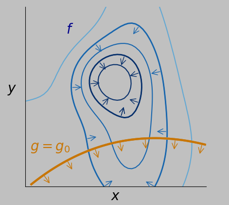
Briefly, Lagrange multipliers are useful when we wish to maximize one function (\(f\), say) while satisfying a constraint involving another function (\(g=g_0\), say, where \(g\) is a function and \(g_0\) is a constant). Let's immediately show a visual example for clarity:

We seek the largest value of \(f\) (shown in blue, with contour loops that get darker with increasing \(f\)) with the constraint that we must stay on the orange planar curve corresponding to the constraint \(g=g_0\).
What point would you select? Does a systematic approach exist? How would you automate this approach? (Produced in Python with this code.)
To obtain a sense of what it means to maximize a function subject to a constraint, assume that our function \(f\) takes as input a 2D location on the \(x\) and \(y\) axes and returns a number on the \(z\) axis, analogous to an elevation or altitude. We pursue this analogy by plotting the contour map of \(f\) above (blue contours), similar to a trail or topographic map, where the output altitude increases in this case as we move to inner contours. Simultaneously, the constraint \(g=g_0\) (the orange planar curve) governs where we are allowed to move. If it weren't for this constraint, of course we'd just pick the peak of \(f\)'s blue mountain; the constraint makes the solution more elusive.
Let's identify a few important aspects of this plot. One is that the gradient of \(f\), or \(\nabla f\) (essentially the multidimensional vector version of a derivative, defined in this context as \(\nabla=\boldsymbol{\hat{x}}\frac{\partial}{\partial x}+\boldsymbol{\hat{y}}\frac{\partial}{\partial y}\), where \(\hat{x}\) points in the \(x\) direction and \(\hat{y}\) in the \(y\) direction) always points toward increasing \(f\) and also always points perpendicular to the \(f\) contour lines, as shown by the vector arrows below, selected for two particular contours of \(f\):
Arrows show the direction of the gradient, which always points perpendicular to contour lines and functions. Blue arrows show the directions of the greatest increase of \(f\) for two contours, and orange arrows show the gradient directions for various locations on the constraint.
In other words, the direction of greatest change is always perpendicular to the direction of no change for a smooth contour. You can try sketching topographic peaks with level contours and considering the direction of maximum slope to prove this result to yourself. Since I love Taylor series expansions, I'll show a more rigorous argument in the box below.
The gradient as the direction of maximum increaseWe seek to show that the gradient of a function (e.g., at a contour curve) always points in the direction of the maximum increase of that function.
Taylor series expansions are generally awesome because they let us approximate \(f(r+\delta r)\) for small \(\delta r\) as
$$f(r+\delta r)=f(r)+f^\prime(r)\delta r+\frac{1}{2!}f^{\prime\prime}(r)(\delta r)^2+\cdots\\+\frac{1}{n!}f^{(n)}(r)(\delta r)^n+\cdots,$$
where the prime symbol indicates the derivative with respect to \(r\) (and the superscript \((n)\) indicates the nth derivative). The vector version, relevant here, is
$$f({\boldsymbol{r}}+{\delta\boldsymbol{ r}})\approx f({\bf r})+(\nabla f)\cdot{\delta\boldsymbol{r}},$$
where the gradient replaces the derivative and the dot product replaces multiplication and where we've dropped all additional terms as insignificant. Since the dot product effectively measures whether two vectors point in similar directions, the last term is maximized when \(\delta\boldsymbol{r}\) points in the same direction as \(\nabla f\), thus maximizing \(f({\boldsymbol{r}}+{\delta\boldsymbol{ r}})\), which is equivalent to saying that the direction of the maximum increase of \(f\) is that of \(\nabla f\).
Regarding the plot above, note that the gradient of the constraint function \(g\), namely, \(\nabla g\), is also perpendicular to the path but in this case shows where we can't go—we're constrained to stay on that path.
Now, there's a contour of \(f\) that tangentially intersects the \(g=g_0\) constraint, and it's not a coincidence that the gradients of the two curves are parallel at that intersection, which of course is the point we seek—the point that maximizes \(f\) while satisfying \(g=g_0\):
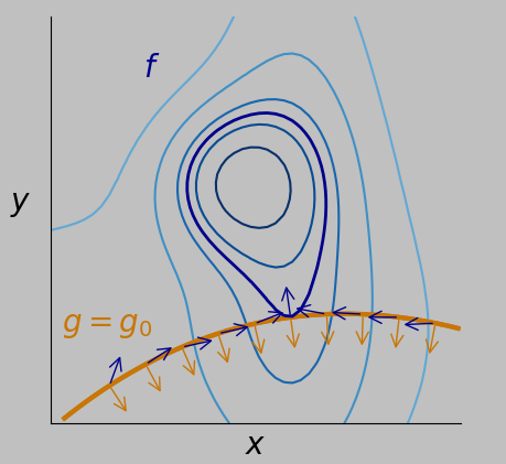
Arrows show the directions of the gradients of \(f\) (blue arrows) and \(g\) (orange arrows) at various points on the constraint \(g=g_0\) (orange curve). The point we seek—which lies on the special contour in dark blue—is the one on the constraint (orange line) where the gradient of the constraint is parallel to the gradient of \(f\). It's at this point that \(f\) is maximized while satisfying \(g=g_0\). This approach provides a systematic way to achieve our objective.
In fact, you can't draw a smooth tangential intersection that doesn't satisfy this property. The mathematical way of expressing that these two gradients \(\nabla f\) and \(\nabla g\) are parallel is
$$\nabla f=\alpha\nabla g,$$
where \(\alpha\) (termed a Lagrange multiplier in this context) is just a scaling constant. In general, \(\alpha\) can be positive or negative. (It would be negative for the condition shown above because at the optimum point, the blue and orange arrows point in opposite directions.)
Here's another way to think of the problem: Since \(\nabla f\) points in the direction of the greatest change, as shown in the box above, we naturally wish to move in this direction to achieve our goal of maximizing \(f\). But when our desired direction \(\nabla f\) is parallel to \(\nabla g\), then we can't do any better. We're stuck: our desired direction is perpendicular to the path that satisfies \(g=g_0\). So we're done—we've optimized our function subject to our constraint.
It's a common theme of these technical notes that we'd like to apply clever results to both move forward and gain engineering intuition. In this case, we could cleverly obtain the same equation and satisfy the original constraint of \(g=g_0\) if we were to proceed as follows:
The Lagrange multiplier method
To maximize \(f\) while satisfying \(g=g_0\), let's re-express the latter relationship as \(g-g_0=0\) and write
$$\mathcal{L}=f-\alpha(g-g_0)$$
(where \({\cal{L}}\) is termed the Lagrangian) and maximize this expression over all \(x\) and \(y\) (written as \(\max_{x,y}{\cal{L}}\)), given that we'll commit to applying the following two operations:
Apply the gradient operator to \({\cal{L}}\) and set the result to zero, which recovers the equation \(\nabla f=\alpha\nabla g\) (as described above) that states that the gradients are parallel. Recall that the gradient is just a set of spatial derivatives, so this process is equivalent to setting the derivative with respect to \(x\) to zero, then with respect to \(y\).
Set the derivative of \({\cal{L}}\) with respect to \(\alpha\) to zero, or \(\frac{\partial {\cal{L}}}{\partial\alpha}=0\), which gives the constraint exactly.
You might note that we can accommodate any number of additional constraints \(g_m=g_{m,0}\) by simply appending \(\sum_m\alpha_m(g_m-g_{m,0})\) to the Langrangian. Wow, I've got chills.
Aren't these two steps equivalent to just individually setting the derivative with respect to every input dimension and every Lagrange multiplier to zero? Yes, exactly, and this is a great way to think about it. In fact, we can express this operation succinctly as
$$\nabla_{x,y,\alpha}{\cal{L}}=0.$$
Remember also that we further wished to obtain \(\max_{x,y}{\cal{L}}\). But wait: doesn't that operation encompass solving \(\nabla_{x,y}{\cal{L}}=0\) anyway because maximizing or minimizing a function involves finding where its derivatives are zero? Yes, except for the case where the maximum lies at infinity, so we would need to throw away those solutions as nonviable. So we find that we can write
$$\max_{x,y}{\cal{L}}~\mathrm{such~that}~\frac{\partial{\cal{L}}}{\partial\alpha}=0.$$
But then we might as well simply write
$$\max_{x,y,\alpha}{\cal{L}}$$
because maximizing any function over \(\alpha\) would entail setting its derivative to zero as well (again, given that we throw away solutions at infinity).
To reiterate, we're happy to allow the Lagrange multiplier \(\alpha\) to assume any value necessary to satisfy the equations obtained from the steps listed above—except infinity. A result of infinity would correspond to no solution.
(This is such an important point that it's useful to re-express it. We can't have an \(x,y\) solution that entails \(g(x,y)\ne g_0\) because that condition violates our fundamental constraint. If \(g > g_0\), then our goal of maximizing the Lagrangian \({\cal{L}}\) could be met with \(\alpha=\infty\), which we've decided is an invalid solution. Conversely, if \(g < g_0\), then we could maximize the Lagrangian \({\cal{L}}\) with \(\alpha=-\infty\), which we've also ruled unacceptable. In this way, the Lagrange multiplier acts as both an essential solution tool and a diagnostic of our optimization solution.)
Thus, the Lagrange multiplier method turns an optimization problem with constraints into several simultaneous equations obtained from steps (1) and (2) that we're free to solve. In turn, the transition from writing \(\nabla_{x,y,\alpha}{\cal{L}}=0\) to writing \(\max_{x,y,\alpha}{\cal{L}}\) allows us to accommodate inequality constraints, which is a very powerful capability. For example, if the constraint were instead \(g\ge g_0\), then we could still use the same Lagrangian as long as we modified the maximization term to read
$$\max_{x,y,\alpha\ge 0}{\cal{L}}.$$
In other words, we previously wished the Lagrange multiplier \(\alpha\) to swing to \(+\infty\) or \(-\infty\) as necessary to invalidate any \({\cal{L}}\)-optimizing solution involving \(g\ne g_0\) because that condition would constitute a constraint violation. Now, however, in the inequality case, we're taking away the capacity for \(\alpha\) to become arbitrarily negative when we maximize \({\cal{L}}\) because it's fine if \(g\ge g_0\).
Isn't this modification clever? Familiarity with this reasoning will enable forward movement.
Let's apply this new familiarity to our problem. By comparing the Lagrangian with the primal form stated above, we can link \(f\) (the function to be maximized or minimized) to \(\frac{1}{2}||\boldsymbol{w}||^2=\frac{1}{2}(\boldsymbol{w}\cdot\boldsymbol{w})\). And we can link the canonical constraint term \(g-g_0\) to our constraint as \((\boldsymbol{w}\cdot\boldsymbol{x_m}+b)y_m-1\). The Lagrangian—customized for our optimization problem, which itself is customized for our classification problem—is therefore
$${\cal{L}}(\boldsymbol{w},b,\alpha)=\frac{1}{2}(\boldsymbol{w}\cdot\boldsymbol{w})-\sum_m\alpha_m\left[(\boldsymbol{w}\cdot\boldsymbol{x_m}+b)y_m-1\right].$$
Because our constraint is expressed as an inequality, we'll maximize \({\cal{L}}(\boldsymbol{w},b,\alpha)\) over all nonnegative \(\alpha\), as discussed in the box above:
$$\max_{\alpha\ge 0}{\cal{L}}(\boldsymbol{w},b,\alpha).$$
And since we specifically wish to minimize \(\frac{1}{2}||\boldsymbol{w}||^2\) by adjusting \(\boldsymbol{w}\) and \(b\), we write as our final form
$$\min_{\boldsymbol{w},b}\max_{\alpha\ge 0}{\cal{L}}(\boldsymbol{w},b,\alpha).$$
We're now ready to differentiate this Lagrangian with respect to our various parameters (as specified in the box above) and see what we find. First, differentiating with respect to \(\boldsymbol{w}\) and setting the result to zero gives
$$\frac{\partial{\cal{L}}}{\partial\boldsymbol{w}}=0\Rightarrow \boldsymbol{w}-\sum_m\alpha_m\boldsymbol{x}_m y_m=0,$$
so that
$$\boldsymbol{w}=\sum_m\alpha_m\boldsymbol{x}_m y_m.$$
(If differentiating the dot product of vectors is new, try expressing the dot product \(\boldsymbol{w}\cdot\boldsymbol{w}\) as \(\sum_i w_iw_i=\sum_i w_i^2\) and bringing the differential operator inside the summation sign. The denominator-layout nomenclature is used.)
Second, differentiating with respect to \(b\) and setting the result to zero gives us
$$\frac{\partial{\cal{L}}}{\partial b}=0\Rightarrow\sum_m\alpha_my_m=0.$$
Finally, it's insightful to verify that if we differentiate the Lagrangian with respect to \(\alpha_m\), then we obtain our original constraint (or at least the equality part of it—the inequality is addressed by our use of \(\max_{\alpha\ge 0}\)).
We've just done everything required to apply the Lagrange multiplier machinery; what remains is to work through the implications and revel in the outcome.
We can expand the terms in the earlier Lagrangian to
$${\cal{L}}(\boldsymbol{w},b,\alpha)=\frac{1}{2}(\boldsymbol{w}\cdot\boldsymbol{w})-\sum_{m}\alpha_m(\boldsymbol{w}\cdot\boldsymbol{x_m})y_m-b\sum_{m}\alpha_my_m+\sum_{m}\alpha_m.$$
The second differentiation outcome above tells us immediately that the third term on the right-hand side is zero, and the first informs us that the first term,
$$\frac{1}{2}(\boldsymbol{w}\cdot\boldsymbol{w})=\frac{1}{2}\sum_{m}\sum_{n}\alpha_m\alpha_ny_my_n(\boldsymbol{x_m}\cdot\boldsymbol{x_n}),$$
is simply one-half the magnitude of the second term
$$-\sum_{m}\alpha_m(\boldsymbol{w}\cdot\boldsymbol{x_m})y_m=-\sum_{m}\sum_{n}\alpha_m\alpha_ny_my_n(\boldsymbol{x_m}\cdot\boldsymbol{x_n}).$$
(If the transition from the dot product to indices seems opaque, it may help to review the definition of the dot product.) Thus, we have
$$\max_{\alpha\ge 0}{\cal{L}}(\alpha)=-\frac{1}{2}\sum_{m}\sum_{n}\alpha_m\alpha_ny_my_n(\boldsymbol{x_m}\cdot\boldsymbol{x_n})+\sum_{m}\alpha_m,$$
the minimization part having disappeared because the parameters \(\boldsymbol{w}\) and \(b\) no longer appear. This last expression is the dual form.
As I cautioned, this content has gotten very math intensive. There's a big payoff:
The kernel trick Importantly, our latest version of the optimization problem, the dual form, includes only the dot products of the input data. Now, the outputs of dot products can be much simpler than their constitutive vectors! Consider, for example, how
$$(2\boldsymbol{i}+3\boldsymbol{j}+4\boldsymbol{k})\cdot(5\boldsymbol{i}+6\boldsymbol{j}+7\boldsymbol{k})$$
works out to simply \(2\cdot 5+3\cdot 6+4\cdot 7=56\), which we can interpret as an objective measure of how much those two vectors point in the same direction, given their length.
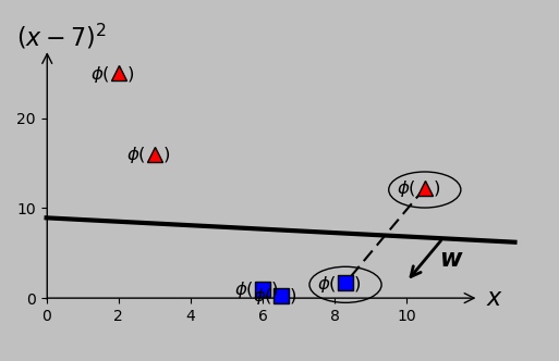
In part 1, overlapping classes prompted us to transform our data from \(x_m\) to \(\boldsymbol{x_m}=\phi(x_m)\). That is, we decided to apply a transformation \(\phi\) to present our data in a higher-dimensional space to achieve linear separability. We didn't know (and still don't know) how to select the best \(\phi\) to use; we selected \(\phi(x)=(x,(x-7)^2)\), but this transformation was straightforward and robust in the sense that we could have subtracted 6.8 or 7.2, for example.
Our latest result indicates that we now need only manipulate \(\phi(x_m)\cdot\phi(x_n)\). The corresponding function for our particular transformation is
$$\phi(x_m)\cdot\phi(x_n)= x_m x_n+(x_m-7)^2(x_n-7)^2,$$
which simply outputs a number. We can represent this scalar function as \(k(x_m,x_n)\), which is called the kernel. (The example shown above is called a decomposable kernel because it's clear what transformation was performed: add a second dimension in which we substract 7 from the data point, and then square the result.)
What if I told you that there are a variety of alternative kernel functions that we could have used that can successfully classify our groups—even our overlapping groups—seemingly on autopilot, without even needing to specify a particular transformation? I'm talking about functions such as
$$k(x_m,x_n)=(x_mx_n+1)^2$$
or
$$k(x_m,x_n)=\exp\left[-(x_m-x_n)^2\right]$$
or
$$k(x_m,x_n)=1-\frac{1}{1-|x_m-x_n|}$$
or
$$k(x_m,x_n)=\min(x_m,x_n),$$
for example, among others. This would be a big win. Happily*, this shortcut is possible and is known as the kernel trick. More on this topic as we work through the process of solving the dual problem (which we expect to produce the same results as solving the primal problem).
*English-language pedants: We are happy; the shortcut is not happy.
The potential advantages of the kernel trick—which are only hinted at above—arguably justify all the challenging mathematical manipulation that's been required up to now. Naturally, we wish to avoid having to develop a customized transformation \(\phi\) for every new data set. We're very close to operating a true support vector machine, now understanding the details of what's actually happening.
For now, let's continue using the arbitrary \(\phi(x_m)=(x_m,(x_m-7)^2)\) transformation that we designed earlier and show that we can solve the optimization problem in the dual form, obtaining the same result as the primal form. We start with the dual-form expression derived above, now incorporating the kernel:
$$\max_{\alpha\ge 0}{\cal{L}}(\alpha)\mathrm{,~where~}{\cal{L}}(\alpha)=-\frac{1}{2}\sum_{m}\sum_{n}\alpha_m\alpha_ny_my_nk(x_m,x_n)+\sum_{m}\alpha_m,$$
$$\mathrm{with~}\sum_m\alpha_my_m=0\mathrm{~(from~the~Lagrange~multiplier~process)},$$
and express it in vector form:
$$\mathrm{maximize~}\left(-\frac{1}{2}\boldsymbol{\alpha}^\mathsf{T}\boldsymbol{y}\boldsymbol{y}^\mathsf{T}\boldsymbol{K}\boldsymbol{\alpha}+\boldsymbol{1}^\mathsf{T}\boldsymbol{\alpha}\right)\\\mathrm{(or,~equivalently,~minimize~}\frac{1}{2}\boldsymbol{\alpha}^\mathsf{T}\boldsymbol{y}\boldsymbol{y}^\mathsf{T}\boldsymbol{K}\boldsymbol{\alpha}-\boldsymbol{1}^\mathsf{T}\boldsymbol{\alpha}\mathrm{)},$$
$$\mathrm{subject~to~}\boldsymbol{\alpha}\ge\boldsymbol{0},$$
$$\mathrm{with~}\boldsymbol{y}^\mathsf{T}\boldsymbol{\alpha}=0,$$
where the kernel matrix \(\boldsymbol{K}\) (also called the Gram matrix) is defined as \(K_{mn}=k(x_m,x_n)\) and where \(\boldsymbol{1}\) is a column vector of ones. It might be helpful—it certainly helps me—to write out these vectors and matrices for a low-dimensional case to see how the indicial notation and the vector notation match up.
Let’s return to the qpsolvers package in Python, applied in part 1, which, we recall, aims to satisfy the following conditions:
$$\mathrm{minimize~}\frac{1}{2}\boldsymbol{u}^\mathsf{T}\boldsymbol{Pu}+\boldsymbol{q}^\mathsf{T}\boldsymbol{u},$$
$$\mathrm{subject~to~}\boldsymbol{Gu}\le\boldsymbol{h},$$
$$\mathrm{with~}\boldsymbol{Au}=\boldsymbol{b}.$$
Comparing the two formulations, we find that we can associate \(\boldsymbol{u}\) with \(\boldsymbol{\alpha}\), \(\boldsymbol{P}\) with \(\boldsymbol{y}\boldsymbol{y}^\mathsf{T}\boldsymbol{K}\), \(\boldsymbol{q}\) with \(-\boldsymbol{1}\), \(\boldsymbol{G}\) with \(-\boldsymbol{I}\) (where \(\boldsymbol{I}\) is the identity matrix, with the negative sign coming from the flipped inequality), \(\boldsymbol{h}\) and \(\boldsymbol{b}\) with \(\boldsymbol{0}\), and \(\boldsymbol{A}\) with \(\boldsymbol{y}^\mathsf{T}\). This we can do.
The code is here. We obtain a solution of \(\boldsymbol{\alpha}\) values (i.e., Lagrange multipliers) of \([0, 0, 0, 0, 0.01719, 0.01719]\).
We know from our previous solution of the primal problem that the input data points \(x_5\) and \(x_6\) are the support vectors in this case. So is \(\alpha\) nonzero only for the support vectors? Absolutely. In fact, this is a classic characteristic of Lagrange multipliers: they're nonzero only when they come into play, when the constraint is being tested. Sound familiar? This rule of thumb is essentially how we think of the support vectors: they're the ones that really matter in the process of classification. To reiterate: support vectors are associated with nonzero Lagrange multipliers.
We can recover the corresponding so-called weights, or \(\boldsymbol{w}\) vector, from the relationship derived earlier:
$$\boldsymbol{w}=\sum_m\alpha_m\boldsymbol{x}_m y_m.$$
The output is \(w_1=-0.038\) and \(w_2=-0.182\), which exactly matches the values we calculated in part 1 by solving the primal form.
And of course we wish to calculate the so-called bias \(b\). Recall that we chose to satisfy \(\boldsymbol{w}\cdot\boldsymbol{x_m}+b=y_m\) exactly at the support vectors, as discussed in the canonical hyperplane section of part 1. And indeed, if we specifically use the support vector \(\boldsymbol{x_5}\) (meaning \(\left(x_5,(x_5-7)^2\right)\)), then we obtain \(b=1.62062\), as verified in the code linked above. If we use \(\boldsymbol{x_6}\), then we obtain \(b=1.62059\). So why not average over all the support vectors (well, it's just these two in this case) to accommodate the slight variations that arise in numerical solutions. This average is \(b=1.62060\), which matches the value of \(b\) calculated in part 1.
But let’s get used to performing classification using the dual form (which emphasizes the Lagrange multipliers \(\boldsymbol{\alpha}\) rather than the weights and bias). Whereas before we performed classification by checking the sign of
$$\boldsymbol{w}\cdot\boldsymbol{x}+b,$$
let's apply the relation \(\boldsymbol{w}=\sum_m\alpha_m\boldsymbol{x_m}y_m\), derived in the Lagrange multipliers section above, to classify new points by the sign of
$$\sum_m\alpha_m(\boldsymbol{x_m}\cdot\boldsymbol{x})y_m+b, $$
or, in vector form, the sign of
$$\boldsymbol{\alpha}^\mathsf{T}\boldsymbol{K^\prime}\boldsymbol{y}+b,$$
where \(\boldsymbol{K^\prime}\) is an \(m\)×\(m\) matrix with diagonal values of \(\boldsymbol{x_m}\cdot\boldsymbol{x}=\phi(x_m)\cdot\phi(x)=k(x_m,x)\); all other entries are zero.
As before, we should expect the result to be exactly –1 for the support vectors of the –1 class and +1 for the support vectors of the +1 class. This output can also be verified through the code linked above. We obtain the same values of \(\boldsymbol{w}\) and \(b\).
So if the output of solving the primal problem is exactly the same as that of the dual problem, why did we bother working through this transformation? The reason is that now that we're aware of the kernel trick, it's not necessary to work with the customized and decomposable kernel \(k(x_m,x_n)=x_m x_n+(x_m-7)^2(x_n-7)^2\) (which we chose by inspection for a relatively simple input data set), which resulted in the following divisions and support vectors:
In fact, we might also obtain satisfactory results with the decomposable kernel \(k(x_m,x_n)=\phi(x_m)\cdot\phi(x_n)=x_m x_n+(x_m-x_0)^2(x_n-x_0)^2\) but with an offset of \(x_0=0\):
In other words, we didn’t need to be careful in choosing an offset of 7 at all. Wow.
And we might also obtain satisfactory results with a kernel of \(k(x_m,x_n)=(x_m\cdot x_n+c)^d\) (the so-called polynomial kernel), where we're free to choose the values of \(c\) and \(d\). For our data, I obtain correct classification with \(c=1\) and \(d=2\), for example:
Actually, anything in the ranges of \(c=1-100\) and \(d=2-4\) allows correct classification. It's remarkable that such a broad range of kernel functions results in correct classification for this dataset that's not linearly separable in 1D.
What's happening here is that a kernel of \((x_mx_n+1)^2\), for example, implies that the data have been transformed into a three-dimensional space: \(\boldsymbol{x_m}=\phi(x_m)=(1,x_m^2,\sqrt{2}x_m)\). (It's good practice to verify that the dot product \(\boldsymbol{x_m\cdot x_n}\) in this case indeed gives the kernel function \(k(x_m,x_n)=(x_mx_n+1)^2\) exactly.) And maybe it shouldn't be surprising, given our successful customized transformation into a second dimension, that machine transformation into three dimensions also provides opportunities for correct classification. The point is that we didn't have to design this transformation or visualize the exact results in three dimensions; we only had to test the input parameters of a certain kernel to secure a valid output.
Furthermore, we might obtain satisfactory results with a kernel of \(\exp\left(-\frac{(x_m-x_n)^2}{2\sigma^2}\right)\) (sometimes called the Gaussian kernel), where we're free to choose the value of \(\sigma\). For our data, I obtain correct classification simply with \(\sigma=1\), for example:
It turns out that anything in the range of \(\sigma=0.5-20\) allows correct classification.
Note how this particular kernel renders almost all of our input data as support vectors. This is a characteristic of so-called radial basis kernels, or kernels that incorporate the distance between points as \(||x_m-x_n||\)—they tend to incorporate much of the complete data set when producing a result.
There's an interesting feature of this Gaussian kernel (and other kernels that contain the exponential function). Recall that the preceding kernel, \(k(x_m,x_n)=(x_m\cdot x_n+c)^d\), could be algebraically shown to represent a transformation into three dimensions (that we didn't have to worry about or visualize). A startling aspect of the Gaussian kernel is that it accesses an infinite-dimensional (!) space—that is (letting \(\sigma=\sqrt{1/2}\) for simplicity), this kernel can be decomposed into
$$\exp\left(-(x_m-x_n)^2\right)=\exp(-x_m^2)\exp(-x_n^2)\exp(2x_mx_n),$$
which is amenable to a Taylor series expansion of the last exponential term to give
$$\exp(-x_m^2)\exp(-x_n^2)\sum_k^\infty\frac{2^kx_m^kx_n^k}{k!}$$
or, dividing the factors evenly,
$$\left(\sum_k^\infty\frac{2^{k/2}x_m^k\exp(-x_m^2)}{\sqrt{k!}}\right)\cdot\left(\sum_k^\infty\frac{2^{k/2}x_n^k\exp(-x_n^2)}{\sqrt{k!}}\right),$$
which is a symmetric dot product of identical functions of \(x_m\) and \(x_n\), revealing that we can, in fact, view the Gaussian kernel as representing an infinite-degree transformation. Although we could never conceivably design every aspect of such a transformation, this kernel effectively applies the operation for us.
And finally, we might obtain satisfactory results with a kernel of \(\min(x_m,x_n)\):
Wait, hold up. This kernel is almost trivial. It doesn't even really do anything; it only selects the lesser of two values. But it still manages to classify our groups correctly? Yes. This output can also be verified using the code code linked above.
This outcome of multiple generic kernels providing correct classification is (in my opinion) as amazing as the finding (presented in part 1) that variable transformations can be used to convert overlapping data into linearly separable data. We're able to obtain accurate classification from a variety of standardized frameworks; although we have to experiment with the input parameters to a certain extent, suitable classification appears to be pretty straightforward, as least for this problem.
But where do these expressions come from? The situation reminds me of that of Bayesian priors, where the joke is that nobody knows and we shouldn’t ask. In this case, we would generally like the Gram matrix \(\boldsymbol{K}\) of the candidate kernel function to be symmetric and to be positive semidefinite (which is sort of the matrix equivalent of \(\ge 0\), although it doesn't imply that any particular element is \(\ge 0\)), corresponding to the so-called Mercer conditions, the exploration of which is outside the scope of this note. In addition, different kernels are favored for different applications; a variety of kernels and their applications are presented here.
Soft margin classification via slack variables
There's one more step before applying an actual support vector machine package to our example data. After all, we always wish to understand what variables we're assigning, and there's a certain parameter (usually designated \(C\)) that plays an enormous role in support vector machine operation and should be discussed.
This discussion introduces the second approach to accommodate overlapping data: slack variables. (The first approach was to transform the input data to a higher dimension, as explored in part 1.) This alternative approach is used when we don't wish to insist on perfect classification. For example, we might have one or a few data points—we could think of them as outliers—that we don't wish to accommodate by changing the classifier function. This situation is reminiscent of the classic issue of model parsimony: how much do we adjust our fit to satisfy every single observation?
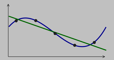
The classic decision of data fitting: do we prefer the simpler model in green (which approximates the data trend and maybe even lies within the error bars of the individual data points) or the more complex model in blue (which fits the data better—indeed, perfectly—but requires more parameters)? There's no right answer—or rather, the answer is situation dependent.
Sometimes we decide that a simpler fit is good enough; equivalently, we decide that the uncertainty in the existing points is large enough that a more complex fit expends unnecessary effort; the simpler fit is probably sufficient to accommodate any new data.
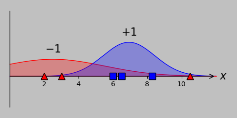
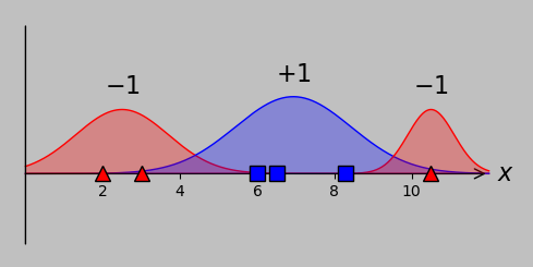
For our toy problem, involving 6 input points and a lack of linear separability, let's consider two possible underlying scenarios that might have produced the data:
Potential Gaussian distributions that might have produced the points we've been using all along. On the left, the red point at 10.5 is an unusual output of a single –1 distribution; on the right, that point arises as a typical output of an additional –1 distribution. The distribution areas for each classification are identical in each case (and are equal to each other).
On the left, we have two distributions, one for the –1 classification (red) and one for the +1 classification (blue). The aberrant red point on the right is an unusual (but not unreasonable) output of the wide distribution of that classification group. To separate the two groups, we would probably wish to use a threshold at approximately \(x=4.5\) and accept the occasional misclassified point.
On the right, we have the situation that the –1 classification arises from two different distributions, one on either side of the +1 classification group. In this case, we would probably wish to enforce thresholds on either side of the blue group; as discussed in part 1, one option to obtain linear separability would be to apply transformation methods such as plotting the data on an additional axis.
In real life, we typically never know the exact originating distribution(s); we can only sample the data and make inferences. We therefore seek a mathematical framework to add rigor to our intuition of using a model of reasonable complexity to get most of the points right without placing too much importance on any one point. Furthermore, we seek a way to tailor our model for different definitions of “most.”
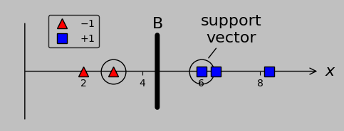
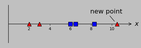
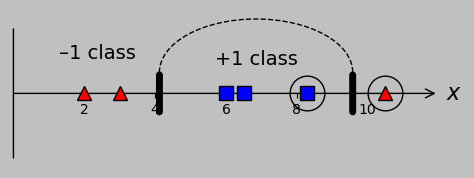
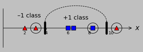
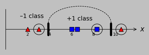
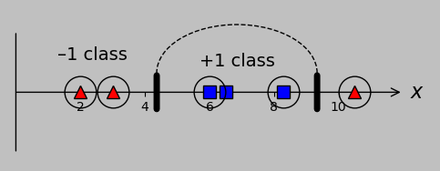
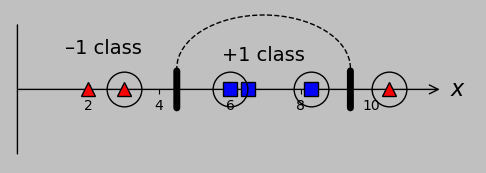
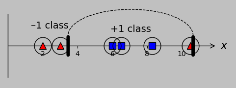
In the support vector machine context, we might decide deliberately to allow misclassification while quantifying the degree of allowed misclassification through so-called slack variables \(\xi_m=\xi(x_m)\), which characterize the distance from the problematic point to the border of the correctly classified points in that group (represented here by the distance from \(x_6\) to the nearest correctly classified point in the –1 class, \(x_2\)):
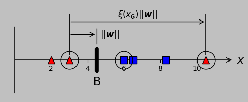
To settle for some degree of misclassification to accommodate outliers, let's define so-called slack variables \(\xi\) that apply to every misclassified point. This approach adds new support vectors (shown encircled, as before): the points that aren't correctly classified.
Let's get our bearings. Taking a look at the figure, we see that the condition \(\xi=0\) corresponds to one of the original support vectors. The condition \(\xi(x_m)>0\) corresponds to a margin violation (but not yet misclassification) for point \(x_m\) lying on the wrong side of the support vector(s) of its class. If \(\xi>1\), then the point is straight-out misclassified (i.e., it's on the wrong side of threshold B in the figure above). If \(\xi>2\), then the point lies within the convex hull of the “wrong” class (because it's as far as or farther than the total margin width from its correct class). What about point \(x_6\) shown above? Here, \(\xi=5\), so this point is totally* misclassified. Clear? Oh, and we're not going to let \(\xi\) be negative; slack variables have meaning only when they're non-negative.
*This adverb added as a salute to Prof. Don Sadoway at MIT, who delights in making fun of textbooks written in California.
This new aspect modifies our optimization problem somewhat, but the difference is easily understandable. Although we choose to allow them, it's probably best to minimize the extent of the slack variables (with a weighting of our choice), so let's add a new term to our expression to be minimized:
$$\mathrm{minimize}~\frac{1}{2}\left(\boldsymbol{w\cdot w}\right)\color{red}{+C\sum_m\xi_m},$$
subject to the constraints
$$(\boldsymbol{w}\cdot\boldsymbol{x_m}+b)y_m\ge 1\color{red}{-\xi_m}$$
$$\mathrm{and}~\color{red}{\xi_m\ge 0.}$$
where the red terms are new. This approach is called 1-norm soft margin classification. (Again, the long phrasing with field-specific jargon might seem opaque until we parse these various terms: the 1-norm corresponds to \(\xi^1=\xi\) in the first line, where the 2-norm would correspond to the alternate—and valid—use of \(\xi^2\); soft classification means that we allow some misclassification; and the concept of the margin was presented and discussed in part 1.)
Note how the former constraint simply matches the definition of \(\xi_m\) shown in the figure above. The latter constraint enforces our earlier decision to require the slack variables to be positive.
It's important to note that this approach of incorporating slack variables can be implemented even if the noisy data actually are separable; maybe we'd like to forego perfect classification (even if it could be trivially obtained) to obtain a larger margin, for example. The relevant adjustment parameter is \(C\), and up to now, we've implicitly set \(C=\infty\); no misclassification has been permitted. That constraint will now be softened by letting \(C\) assume a finite (but always positive) value.
A small \(C\) value allows our original fitting constraints to be easily ignored, corresponding to the straight green line in the parsimony plot above. A large \(C\) value places more weight on a smaller but more “successful” margin (in the sense of less misclassification). Again, \(C=\infty\) imposes a hard margin, corresponding to our strategy up to this point.
The corresponding Lagrangian, which unfortunately seems to be getting more complex by the moment, is now
$${\cal{L}}(\boldsymbol{w},b,\color{red}{\xi},\alpha,\color{red}{\beta})=\frac{1}{2}(\boldsymbol{w}\cdot\boldsymbol{w})\color{red}{+C\sum_m\xi_m}-\sum_m\alpha_m\left[(\boldsymbol{w}\cdot\boldsymbol{x_m}+b)y_m-1\color{red}{+\xi_m}\right]\\
\color{red}{-\sum_m\beta_m\xi_m},$$
and we seek to find
$$\min_{\boldsymbol{w},b,\color{red}{\xi}}\max_{\alpha\ge 0,\color{red}{\beta\ge 0}}{\cal{L}}(\boldsymbol{w},b,\color{red}{\xi},\alpha,\color{red}{\beta}),$$
where the terms in red have all arisen through our allowance of a soft margin. Fortunately, this complexity is going to evaporate quickly.
As specified by the Lagrange multiplier technique described earlier, we'll be evaluating \(\nabla_{w,b,\xi,\alpha,\beta}=0\). Note in particular that one of the new equations,
$$\frac{\partial{\cal{L}}}{\partial \xi}=0,$$
yields \(C-\alpha-\beta=0\). Since \(\beta\ge 0\), we must have \(\alpha\le C\). Applying this and all the other Lagrange-derived expressions as described earlier, we find that many terms cancel out again, producing the following dual form:
$$\max_{0\le\alpha\color{red}{\le C}}{\cal{L}}(\alpha)=-\frac{1}{2}\sum_{m}\sum_{n}\alpha_m\alpha_ny_my_nk(x_m,x_n)+\sum_{m}\alpha_m.$$
where the only new element is shown in red. (That is, all terms involving \(w\), \(b\), \(\xi\), and \(\beta\) end up disappearing, and so the dual form in this case depends only on the Lagrange multipliers, the input data and output classifications, and the kernel—as before—in addition to the weighting parameter \(C\).)
Such a small change, but it provides substantial accommodation in practical classification problems. In practice, this change simply means that the Lagrange multipliers can't exert their influence in an unlimited way to accommodate the potential for misclassification. And so we obtain a new group of Lagrange multipliers and support vectors: whereas before we classified the Lagrange multiplier results \(\alpha_m\) as zero (non-support vectors) or nonzero (support vectors), we can now add the new class of \(\alpha_m=C\) for support vectors that lie on the wrong side of their margin boundary, as graphically shown above, which we can forgive to some varying degree by our selection of \(C\).
To be clear, we now have three potential situations:
\((\alpha_m=0)\): The point has been correctly classified, and it wasn't really any effort. In other words, the point isn't a support vector. There is no slack variable (or we could say that \(\xi_m=0\)).
\((0\lt\alpha_m\lt C)\): The point has been correctly classified, and its Lagrange multiplier came into play; in other words, the point is a support vector because it played a part in setting the hyperplane location and orientation. This type of support vector, which lies on the margin, is called an unbounded or free support vector. Here, too, we could say that there is no slack variable, or \(\xi_m=0\).
\((\alpha_m=C)\): In our optimization effort, the Lagrange multiplier has hit its preassigned limit, and the point lies on the wrong side of its margin (\(\xi_m>0\)). The point might still be correctly classified, however, as long as \(\xi_m\) doesn't exceed 1. (This condition corresponds to the case where making this point a free support vector would produce a margin width too small for our taste.) But if \(\xi_m>1\), then the point is misclassified. In any case, this point is also a support vector (because this point is problematic, which is another way of being important), and it's specifically called a bounded support vector because it lies on the wrong side of its appropriate margin.
A further reiteration: if we had used the unforgiving value of \(C=\infty\) (which was the default up to now), then the Lagrange multiplier for one or more points would have swung to infinity, thus invalidating the solution. Augmenting the framework to allow a finite \(C\) allows us to accept less-than-perfect classification.
Operating a support vector machine—finally
With this intuitive understanding of key machinery (maximizing the margin and accommodating misclassification) and parameters (input data, output classifications, support vectors, and Lagrange multipliers), we're now ready to implement a real support vector machine package. A suitable choice is the sklearn.SVM package. The corresponding code to implement this package for our problem is here.
That code includes the details to reproduce the results obtained earlier (specifically, we define a function my_kernel that subtracts 7 and squares the result, corresponding to our \(\phi\) transformation). For very large values of \(C\), the results are identical to those obtained from the more manual approach with the qpsolvers package, as we would expect, until we reduce the parameter \(C\) to 0.001 or below; beyond this threshold, there's insufficient driving force to try to fit the additional data point in the –1 classification.
Specifically, for our original transformation \(\phi(x_m)=(x_m,(x_m-7)^2)\) and associated decomposible kernel \(k(x_m,x_n)=x_mx_n+(x_m-7)(x_n-7)\), here's what the results look like for very large \(C\):
which matches the previous results of correct classification. And here's what the results look like if we reduce \(C\) to 0.001:
So with these settings, we don't achieve correct classification, even with the use of a kernel and slack variables, because this low \(C\) value doesn't sufficiently penalize misclassification.
A gallery of classification results
(In development. Survey several data arrangements, kernels, and C values.)
(TBD)
What still needs to be covered
Time for reflection. We now have a much better sense of how to accommodate overlapping data sets and outliers; we can implement both data transformation (simplified by the kernel trick) and slack variables to allow misclassification. And we've actually applied support vector software! However, the presence of all of these new knobs to adjust leaves us with some questions:
How do we objectively characterize or evaluate the performance of a support vector machine? (This is the purview of scoring metrics.)
With all these new choices, how do we identify the best kernel and kernel parameters and the best misclassification parameter \(C\)? (This is the purview of cross validation.)
Importantly (for our aim), how do we switch from classification to regression, and how do we choose to represent a Raman spectrum as a vector in an efficient way for regression?
Part 2 ends here. To address these considerations, part 3 will cover scoring, cross validation, and the transition from classification to regression, and it will cover principal component analysis to succinctly express spectral data.