Motivated by the cool graphics in these answers to a Stack Exchange question, I wanted to show a fitting curve that boings into place as if pulled by individual tethers to each data point (full code here, discussion of various aspects to follow).
Could the motion look like that of an underdamped oscillator, a system commonly encountered in the undergrad STEM curriculum?
In this simple system, a spring (i.e., a perfectly elastic element) is connected in parallel with a damper or dashpot (i.e., a perfectly viscous component). A mass is attached to the free end. When this end is pulled and released, it boings back into place with oscillation—that is, if it’s underdamped, which in practice means that \(c<2\sqrt{km}\), where the spring stiffness is \(k\) (measured in \(\mathrm{N\,m^{-1}}\) in SI units), the damper viscosity is \(c\) (\(\mathrm{N\,m^{-1}\,s^{-1}}\)), and the mass of the mass is \(m\) (\(\mathrm{kg}\)). Here, I selected \(k=4\,\mathrm{N\,m^{-1}}\), \(c=1.2\,\mathrm{N\,m^{-1}\,s^{-1}}\), and \(m=1\,\mathrm{kg}\) for pleasing results.
So how do we find the governing equation for this motion?
The wonderful world of spring-mass-damper systems
If we wished to know the displacement \(x(t)\) over time \(t\) of the underdamped spring-mass-damper system after pulling it out of equilibrium (to a distance \(x_0\)) and letting it go, we could just do an online search for the correct equation, which turns out to be the intimidating-looking
$$x(t)=x_0\exp(-z\omega_nt)\left[\cos(\omega_dt)+\frac{z}{\sqrt{1-z^2}}\sin(\omega_dt)\right],$$
where the so-called damping coefficient \(z=c/(2\sqrt{km})\), the natural frequency \(\omega_n=\sqrt{k/m}\), and the damped natural frequency \(\omega_d=\omega_n\sqrt{1-z^2}\).
Alternatively, we could derive that equation ourselves and, in the process, review some rich concepts in the fields of dynamics, viscoelasticity, vibrations, control theory, and integral transforms.
Let’s start with a force balance of the spring-mass-damper assembly shown above and assume that downward displacements and forces are positive. For the spring, Hooke’s Law tells us that the restoring force \(F\) scales with the displacement \(x\), so \(F_{\mathrm{spring}}=-kx\). Dampers are a little different: the resisting force scales with the rate of displacement, so \(F_{\mathrm{damper}}=-c\dot{x}\), where the dot indicates the first time derivative. In other words, dampers resist movement much more when pulled at rapid rates, whereas springs are rate independent. Oh, and springs tend to return to their original position when released, whereas dampers just sit there. Finally, masses follow Newton’s Third Law as \(F=m\ddot{x}\), where the double dot indicates the second time derivative—forces make masses accelerate.
For generality, let’s assume that we apply a downward force \(F(t)\) to the platform (up to now, this applied force was assumed to be zero), and let’s note that the spring and damper are connected in parallel, so their forces add. OK.
By summing the vertical forces acting on the mass and applying Newton’s Third Law, we obtain
$$F(t)-kx(t)-c\dot x(t)=m\ddot{x}(t)$$
or
$$F(t)=m\ddot{x}(t)+c\dot{x}(t)+kx(t),$$
which is an ordinary differential equation. We’d like to solve this equation to obtain, for example, \(x(t)\) as a function of \(x_0\) (the initial displacement), \(\dot{x}_0=v_0\) (the initial velocity), and \(F(t)\). If you’ve read other technical notes on this site, you know that I love integral transforms because they change differential equations (even integrodifferential equations) into algebraic equations that can be much easier to solve. The Laplace transform, for example, is great for solving time-dependent differential equations of this type we have here.
The strategy is as follows: we can apply the Laplace transform (denoted by \({\cal{L}}\)) to the time-domain differential equation to obtain an algebraic equation in the Laplace domain (the so-called \(s\) domain), solve that equation, and apply the inverse transform (\({\cal{L}}^{-1}\)) to determine the solution in the time domain. A table of Laplace transforms is useful here to let us review the relevant transform pairs.
For example, we can write the Laplace transforms of functions such as \(x(t)\) and \(F(t)\) as just \(x(s)\) and \(F(s)\), respectively, which really means that we’ll hold off on determining their transforms until they’re defined. Constant coefficients such as \(k\), \(c\), and \(m\) simply carry through—so we would write $${\cal{L}}[kx(t)]=kx(s),$$ for example. Finally, the Laplace transform of a time derivative is $${\cal{L}}[\dot{x}(t)]=sx(s)-x_0,$$ where \(x_0\) is the initial condition at time 0.
(The time derivative \(\dot{x}(t)\) of the displacement is the velocity, of course. Using the same strategy, now knowing the Laplace transform of the velocity, can you work out the Laplace transform of the acceleration \(\ddot{x}(t)\), knowing that the acceleration is the time derivative of the velocity? It’s $${\cal{L}}[\ddot{x}(t)]=s^2x(s)-sx_0-v_0,$$ where \(v_0=\dot{x}\) is the initial velocity at time 0.)
Applying all of these guidelines to derive the equation of the spring-mass-damper system in the Laplace domain, we obtain
$$F(s)=m[s^2x(s)-sx_0-v_0]+c[sx(s)-x_0]+kx(s)$$
or
$$F(s)=x(s)(s^2m+sc+k)-(smx_0+mv_0+cx_0)$$
or
$$x(s)=\frac{F(s)+smx_0+mv_0+cx_0}{s^2m+sc+k}.$$
Look at that. We have an equation for the displacement, as we hoped, in terms of any applied force and any initial displacement and any initial velocity. Of course, the equation is still in the framework of the Laplace domain, which isn’t immediately useful in terms of simply plotting the response. But it’s a good start.
To build up intuition in understanding the spring-mass-damper response as determined using the Laplace transform, let’s consider various adapted versions of this equation in ten parts.
1. What if the mass \(m\) and damping coefficient \(c\) are actually zero and the initial displacement \(x_0\) and velocity \(v_0\) are also zero? Then
$$x(t)={\cal{L}}^{-1}[x(s)]={\cal{L}}^{-1}\left(\frac{F(s)}{k}\right)=\frac{F(t)}{k},$$
which is just Hooke’s Law again (but without the minus sign because the force is the applied force, not the restoring force).
2. What if there’s no force, but there’s an initial displacement, and there’s a mass and spring but no damper? We then have
$$ x(t)={\cal{L}}^{-1}[x(s)]={\cal{L}}^{-1}\left(\frac{smx_0}{s^2m+k}\right)={\cal{L}}^{-1}\left(\frac{sx_0}{s^2+k/m}\right).$$
A glance at the Laplace transform table reveals that
$${\cal{L}}[\cos(at)]=\frac{s}{s^2+a^2},$$
so the reverse case (with \(a^2=k/m\)) also holds:
$$x(t)=x_0\cos\left(\sqrt{\frac{k}{m}}t\right)$$
which indicates that a released spring-mass system simply oscillates with a resonant angular frequency (denoted by \(\omega_n\), as noted above) of \(\sqrt{k/m}\):
3. What if we remove the mass from the previous system but reinsert the damper? Then we have
$$ x(t)=\cal{L}^{-1}[x(s)]=\cal{L}^{-1}\left[\frac{cx_0}{sc+k}\right]=\cal{L}^{-1}\left[\frac{x_0}{s+k/c}\right].$$
Another glance at the Laplace transform table reveals that
$${\cal{L}}[\exp(at)]=\frac{1}{s+a},$$
so the reverse case (with \(a=k/c\)) also holds:
$$x(t)=x_0\exp(-kt/c),$$
which indicates that the massless platform is simply drawn back to its original position through exponential decay, with the speed progressively slowing as the final position is approached:
Note how substantially different the time-dependent responses are for relatively simple changes in the original system/equation. The already-established machinery of the Laplace transform automatically handles these changes (as long as we can find an inverse transform—the case is similar to that of integration vs. differentiation, where we can’t integrate something unless we already know what we can differentiate to get what we have).
4. Hey, just to try it out, what if both the mass and the damper aren’t present, and we start out with only a stretched spring? We end up with \(x(s)=0\), corresponding to \(x(t)=0\), and this result reminds us that regardless of the initial displacement or velocity, an ideal spring returns to its equilibrium position instantaneously. There’s just nothing that would make it either slow down or overshoot and oscillate.
5. Let’s now consider some different types of loads. One possibility is to hang a small mass on the platform, corresponding to a constant gravitational force. For me, a very counterintuitive aspect of the Laplace transform (resulting in hours of frustration) is that it transforms a constant (e.g., \(F_0\)) not into \(F_0\) but into \({\cal{L}}(F_0)=F_0/s\) (I always forget the factor of \(s\), which arises from the implicit multiplication by the unit step). To reiterate, additive constants are divided by \(s\) in the process of Laplace transformation.
(Is there anything that gets Laplace transformed into a constant? Yes: an impulse, and this is another important type of loading that we’ll discuss next, in part 6.)
So if we suddenly apply a load \(F_0\) to a spring-damper system (no mass), then the response (in the Laplace domain) is
$$x(s)=\frac{F_0}{s(sc+k)}=\frac{F_0/k}{s}-\frac{F_0sc/k}{sc+k}=\frac{F_0/k}{s}-\frac{F_0s/k}{s+k/c},$$
where we’ve used some algebraic manipulation to produce simpler denominators (this technique, often inflicted on mechanical engineers studying vibration and electrical engineers studying circuits, is called partial fraction expansion). Inverse transformation provides the time-domain displacement:
$$x(t)=\frac{F_0}{k}-\frac{F_0}{k}\exp(-kt/c)=\frac{F_0}{k}\left[1-\exp(-kt/c)\right],$$
which corresponds to a smooth, exponentially decaying approach to the equilibrium condition of applying the load to the spring alone
(Certain rules of thumb are emerging. One is that a mass is necessary for free oscillation. Inertia is necessary for free oscillation. Another is that long-term equilibrium conditions correspond to the case of any dampers not even participating. Over long times, dampers don’t really matter and in fact essentially disappear. But the converse also applies: Over short times, dampers are nearly rigid. If a damper completely bridges some portion of a viscoelastic assembly, you’ll never see that portion move instantaneously—aside from the special case of an impulse load, which idealizes loading over a short time as occurring over infinitesimal time.)
6. Next is the important case of the impulse load. Impulses are interesting because first, they’ve been likened to striking the system with a hammer, which is pretty cool, and second, their Laplace transform is simply their scalar magnitude.
For an impulse strike of strength \(\delta_0\), the solution in the Laplace domain (from taking the above general equation
$$x(s)=\frac{F(s)+smx_0+mv_0+cx_0}{s^2m+sc+k}$$
and setting \(x_0=v_0=0\) and inserting \(F(s)=\delta_0\)) is
$$x(s)=\frac{\delta_0}{s^2m+sc+k}.$$
Scanning the list of Laplace transform pairs, we see that
$${\cal{L}}[\exp(-at)\sin(bt)]=\frac{b}{(s+a)^2+b^2},$$
suggesting that we might transform our denominator into a perfect square plus another term. And we can. Let’s set \(z=c/2(\sqrt{km})\) and note that we then have
$$x(s)=\frac{\delta_0/m}{s^2+2sz\omega_n+\omega_n^2}=\frac{\delta_0}{m\omega_n\sqrt{1-z^2}}\left(\frac{\omega_n\sqrt{1-z^2}}{(s+z\omega_n)^2+\omega_n^2(1-z^2)}\right),$$
where we’ve used the definition of the natural frequency \(\omega_n=\sqrt{k/m}\). The advantage of this more complex expression is that the term in big parentheses corresponds to the abovementioned Laplace transform pair with \(a=z\omega_n\) and \(b=\omega_n\sqrt{1-z^2}\). It’s important for solution consistency that the radicand, the term inside the radicals, is positive—in fact, this turns out to be the dividing line between oscillatory (\(z<1\)) and nonoscillatory (\(z>1\)) behavior. For convenience, let’s further define \(\omega_d=\omega_n\sqrt{1-z^2}\). (You may remember these definitions from earlier, before we reviewed how to implement the Laplace transform.) Now we can write
$$x(s)=\frac{\delta_0}{m\omega_d}\left(\frac{\omega_d}{(s+z\omega_n)^2+\omega_d^2}\right),$$
allowing straightforward inverse Laplace transformation to
$$x(t)=\frac{\delta_0}{m\omega_d}\exp(-z\omega_n t)\sin(\omega_dt).$$
Right on. Here’s what that damped oscillatory motion looks like for an impulse load and the same parameters as before:
The ratio \(x(s)/F(s)\) (i.e., the response in terms of the load) is known as the
transfer function of the system. Since the transfer function is the response to a unit impulse load, if we strike a linear system with a hammer (in a matter of speaking) and then measure the response with sufficient accuracy, we now in theory know the response of the system to
any given input.
7. At this point, it’s not much more effort to derive for ourselves the equation given far above for a spring-mass-damper system that’s been pulled out of position and allowed to spring—and oscillate—back into its equilibrium state.
In the absence of a force or initial velocity, the displacement (in the Laplace domain) for the spring-mass-damper system with an initial displacement \(x_0\) is
$$x(s)=\frac{smx_0+cx_0}{s^2m+sc+k}.$$
Based on our experience so far, division by \(m\) and a shift to more convenient variables gives
$$x(s)=\frac{sx_0+2z\omega_n x_0}{s^2+2sz\omega_n+\omega_n^2}.$$
Based on the insight built up from the previous 6 examples, we skillfully convert the denominator to give
$$x(s)=\frac{sx_0+2z\omega_n x_0}{(s+z\omega_n)^2+\omega_d^2}.$$
Let’s add one more transform pair, which again can be found in a table of Laplace transforms:
$${\cal{L}}[\exp(-at)\cos(bt)]=\frac{s+a}{(s+a)^2+b^2},$$
We see that we can decompose \(x(s)\) into
$$x(s)=\frac{sx_0}{(s+z\omega_n)^2+\omega_d^2}+\frac{2z\omega_n x_0}{\omega_d}\left(\frac{\omega_d}{(s+z\omega_n)^2+\omega_d^2}\right),$$
which has the inverse transformation
$$x(t)=x_0\exp(-z\omega_nt)\left[\cos(\omega_dt)+\frac{z}{\sqrt{1-z^2}}\sin(\omega_dt)\right],$$
which is exactly the equation given at the top of this box. This expression is the one we were looking for—the one that guides the dynamic motion of a curve that boings into place, as used in the code following this box. For more insight, continue reading to see how spring-mass-damper systems respond to oscillatory inputs.
8. Earlier, we noted that the unit impulse response in the time domain is exactly the transfer function that completely describes a linear system. Instead of striking the system and looking at the time-domain response, we alternatively could apply sinusoidal inputs of various frequencies and look at the magnitude and phase response. The result is the same: complete system characterization.
We can express such a sinusoidal input as \(F(t)=F_0\exp(i\omega t)\) (where \(\omega\) is the angular frequency of oscillation and \(i\) is the imaginary unit), relying on the Euler relation \(\exp(ix)=\cos(x)+i\sin(x)\). The introduction of the imaginary unit is for ease of calculation only; since physical quantities can take only real values, we’ll commit to discarding the imaginary portion to obtain the actual response in the time domain. Furthermore, for some complex response \(a+ib\), we’ll calculate the magnitude as \(\sqrt{a^2+b^2}\) and the phase lag as \(\tan^{-1}(b/a)\).
Why switch from straightforward trigonometric functions to an exponential involving imaginary numbers? Because (for a linear system) the response also oscillates as \(x(t)=x_0\exp(i\omega t)\)—in fact, every mobile component in the system is moving with an angular frequency of \(\omega\). This is useful.
In particular, recall that the time derivative of \(\exp(i\omega t)\) is \(i\omega\exp(i\omega t)\). We can therefore replace \(\dot{x}(t)\) by \(i\omega x(t)\) (and, in turn, \(\ddot{x}(t)\) by \(-\omega^2x(t)\)). Our original force balance differential equation
$$F(t)=m\ddot{x}(t)+c\dot{x}(t)+kx(t)$$
becomes the algebraic equation
$$F_0\exp(i\omega t)=(-\omega^2m+i\omega c+k)x_0\exp(i\omega t),$$
corresponding to a transfer function of
$$\frac{x_0}{F_0}=\frac{1}{-\omega^2m+i\omega c+k}.$$
To work through the implications of this expression, let’s first ignore damping to obtain
$$\frac{x_0}{F_0}=\frac{1}{-\omega^2m+k},$$
or, dividing by \(m\),
$$\frac{x_0}{F_0}=\frac{1/m}{-\omega^2+\omega_n^2},$$
which has a denominator of zero if \(\omega=\omega_n=\sqrt{k/m}\). We found earlier that \(\omega_n\) is the characteristic frequency (termed the natural frequency) of an undamped spring-mass system, and we now confirm that it is in fact the resonant frequency. The zero-denominator condition is what’s called a pole in control theory, generally indicating that a displacement or some other response parameter grows without limit. In practice, the system flies apart.
So-called Bode plots give insight into frequency-dependent systems because they describe the complete response in terms of the amplitude and phase of the output wave, among other advantages. The amplitude gives the maximum extent of the response, and the phase lag indicates how unsynchronized the output is from the input.
The Bode plots for our particular spring-mass system emphasize the extreme results of excitation near the natural frequency \(\omega_n\) and the associated sudden phase change:
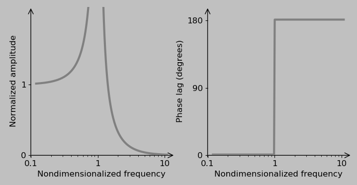
The nondimensionalized frequency plotted on the x-axis of the charts is \(\Omega=\omega/\omega_n\), making the spring-mass frequency response look like
$$\frac{x_0}{F_0}=\frac{1/(m\omega_n^2)}{1-\Omega^2},$$
Note again the pole at \(\Omega=1\).
Qualitatively, here’s what’s happening:
At very low frequencies (\(\omega \rightarrow 0\) and \(\Omega\rightarrow 0\)), the mass follows the driving force precisely: the normalized amplitude is one, and the phase lag is zero. As the spring is extending, the entity applying the force is doing work on the system; as it’s contracting, this energy transfer is reversed. (The system only stores energy; no energy is dissipated at any frequency because no damper is present.)
At very high frequencies, the mass hardly moves at all because its inertia prevents it from keeping up with the wildly oscillating force. In fact, the motion of the mass is perfectly out of phase with the force, which (interestingly) means that the force is always acting to draw the mass back to its static equilibrium position.
At \(\omega=\omega_n\), resonance occurs. Although the phase lag is undefined at this frequency for the spring-mass system, we can imagine the sinusoidal force peaking exactly when the mass is already at its greatest speed, which maximizes the excitation effect.
So that’s pretty cool. Now, if the damping isn’t zero, then the transfer function expressed with convenient variables is
$$\frac{x_0}{F_0}=\frac{1/m}{-\omega^2+2i\omega z\omega_n+\omega_n^2}=\frac{1/(m\omega_n^2)}{-\Omega^2+2iz\Omega+1}.$$
The factor of \(2iz\Omega\) now prevents the denominator from ever going to zero. (This model is more representative of real systems, all of which exhibit some degree of damping, of course, although real systems can still fly apart under resonance.)
The imaginary unit \(i\) might seem problematic because no real physical phenomenon can have an imaginary component. We got into this situation by committing to considering only the real part of \(\exp(i\omega t)=\cos(\omega t)+i\sin(\omega t)\). In practical terms, the imaginary part simply means that the system is storing some out-of-phase energy that’s not apparent from the real part of \(x_0/F_0\). (If you imagine a sinusoid as the horizontal projection of a rotating arrow, then the imaginary component corresponds to the vertical projection.) As noted earlier, the magnitude of a system with response \(a+ib\) is \(|a+ib|=\sqrt{a^2+b^2}\). It follows that for a function \(\frac{a+ib}{c+id}\), the magnitude is
$$\left|\frac{a+ib}{c+id}\right|=\frac{\sqrt{a^2+b^2}}{\sqrt{c^2+d^2}},$$
which you can prove to yourself by multiplying the denominator by \(c-id\) and working from there. The amplitude of the complete spring-mass-damper system excited by a force is therefore
$$\left|\frac{x_0}{F_0}\right|=\frac{1/(m\omega_n^2)}{\sqrt{(1-\Omega^2)^2+(2z\Omega)^2}},$$
with the corresponding Bode plots
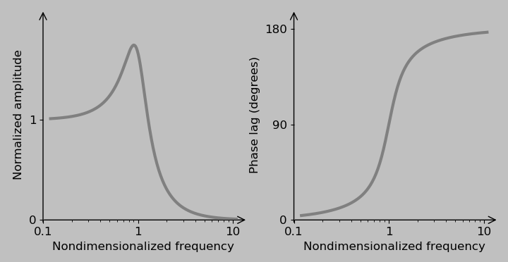
These Bode plots are slightly “softened” versions of those of the spring-mass system in which the damper prevents the system from ever going to infinity and the phase lag is a smoother and continuous function.
For an excitation frequency of half of the natural frequency, the corresponding dynamic response looks like this:
9. Let’s now check out another type of loading, oscillatory seismic excitation, which we’ll illustrate straightaway:
Here, instead of a force driving the mass directly, the base moves to drive motion in the mass through the spring and damper. And actually, thinking about the action of the base on the mass is the key: Let’s denote the position of the base by \(y\) so that \(F(t)=c(\dot{y}-\dot{x})+k(y-x)\). A force balance gives
$$c\dot{y}(t)+ky(t)=m\ddot{x}(t)+c\dot{x}(t)+kx(t),$$
which—after replacing each derivative by \(i\omega\) to examine purely oscillatory behavior and simplification into more convenient variables—gives (by dividing by \(m\) and \(c\) and then \(\omega_n^2\))
$$\frac{x_0}{y_0}=\frac{2iz\Omega+1}{-\Omega^2+2iz\Omega +1},$$
which has a magnitude of
$$\left|\frac{x_0}{y_0}\right|= \frac{\sqrt{(2z\Omega)^2+1}}{\sqrt{(1-\Omega^2)^2+(2z\Omega)^2}}.$$
Note how similar the Bode plots appear for the two cases of direct force excitation and seismic excitation. Actually, the behaviors at the low-frequency and high-frequency extremes are essentially identical.
10. The situation is quite different in the case of a rotating imbalance, another classic way of exciting a system:
Here, we have a spinning second mass whose rotational acceleration imparts a sinusoidal vertical force acting on the spring-mass-damper system. (Horizontal motion is assumed to be constrained, so the associated sinusoidal horizontal force has no effect.) This rotation-based vertical force scales with the square of the spinning frequency \(\omega\) (i.e., \(|F(t)|\sim\omega^2\)), so the magnitude of the transfer function can be immediately written (for a small rotating mass) as
$$\left|\frac{x_0}{F_0}\right|=\frac{\omega^2}{|-\omega^2m+iwc+k|}$$
or
$$\left|\frac{x_0}{F_0}\right|=\frac{\omega^2/m}{|-\omega^2+2i\omega z\omega_n+\omega_n^2|}$$
or
$$\left|\frac{x_0}{F_0}\right|=\frac{\Omega^2/m}{|-\Omega^2+2iz\Omega+1|}$$
or
$$\left|\frac{x_0}{F_0}\right|=\frac{\Omega^2/m}{\sqrt{(1-\Omega^2)^2+(2z\Omega)^2}}.$$
In this case, at low frequencies, the response is nearly zero because the small mass rotating at a small frequency has almost no influence. At higher frequencies, the rotational acceleration starts to excite the main mass. At still higher frequencies, indeed, very high frequencies, does the response drop to zero as it did in the other examples? It does not. The imbalance rotational acceleration—and associated applied force—just keeps scaling up to match the mass inertial resistance.
This material represents a large initial chunk of an undergraduate vibrations and control class in mechanical engineering. It can be effectively ported over to an analog circuits class in electrical engineering, where the compliance (reciprocal stiffness) of the spring corresponds to a capacitance, the viscosity of the damper corresponds to a resistance, the mass corresponds to an inductance, speed corresponds to current, and force corresponds to voltage (also known as electromotive force).
So that’s what it takes to derive the constitutive equation of an object that boings into place.
The discussion now moves to the code. For the current demonstration in Python, involving the motion into place of a fitting line and then a fitting polynomial, the following requirements seemed appropriate:
- Generate an arbitrary number of points with an underlying function (if desired) and some degree of randomness (if desired).
- Fit a line and also a polynomial (of arbitrary degree) to the data, and store this information.
- Show a line popping up (from an arbitrary location) to pass through the middle of the data.
- Show the line rotating into the line position of best fit.
- Show the line transforming into the polynomial fit.
- Link the line/curve to the data points with thin perpendicular connecting lines to give the visual effect that the fit is being pulled into place.
- Boing the line into each new configuration in that cool underdamped oscillatory style.
OK, let’s get into the program construction. Again, the full code is here. The strategy is as follows, from goal to necessary code:
- Since we want an animation that progresses from one type of behavior to another, let’s give names to these “scenes” and specify their durations.
- Each scene involves one or more lines or curves that move and fade in or out as necessary.
- The movement follows the underdamped oscillatory function but also depends on the data points and other lines/curves, so let’s define additional functions that return important relationships such as the distance from a point to a line, the position of the closest point on a line or curve, and the best polynomial fit to multiple points.
- We need to carefully keep track of the total time and time in each scene so that the fading is synchronized and
aesthetically pleasing.
Let’s go through the code unit by unit. First, we import the necessary packages: matplotlib (including FuncAnimation) for graphics (and animation), numpy for various mathematical manipulations, and sympy for some symbolic differentiation that helps when determining the closest point on a polynomial from a data point.
(Side note: I’ve read that the code import [package] as * is not recommended, as a prefix is useful to avoid confusing functions from different packages. However, I get error messages for commands like sympy.Poly, so sympy is imported here without a prefix. I must have misunderstood something.)
from matplotlib import pyplot as plt
import numpy as np
from sympy import *
from matplotlib.animation import FuncAnimation
print("Ready")
Then follows a series of figure creation and customization commands. Only the first is essential to make the figure; the others apply a personal house style, including an aspect ratio of unity and a background color that matches this website.
fig, ax = plt.subplots(figsize = (4, 4))
ax.set_aspect(1)
plt.rc(’font’, size = 16)
marker_style = dict(linestyle = ’none’, markersize = 10,
	markeredgecolor = ’k’)
plt.box(on = None)
fig.set_facecolor(’#c0c0c0’)
plt.rcParams[’savefig.facecolor’] = ’#c0c0c0’
ax.spines[’bottom’].set_position(’zero’)
ax.spines[’left’].set_position(’zero’)
Next, we plot the axes and set some parameters to get the ticks and margins just right:
(min_plot, max_plot) = (0, 10)
plt.xticks(np.arange(min_plot, max_plot + 1, 2), fontsize = 10)
plt.yticks(np.arange(min_plot, max_plot + 1, 2), fontsize = 10)
plt.xlim([min_plot - 1, max_plot + 1])
plt.ylim([min_plot - 1, max_plot + 1])
ax.annotate(’’, xy = (min_plot, max_plot + 1),
	xytext = (min_plot, min_plot - 0.1),
	arrowprops = {’arrowstyle’: ’->’, ’lw’: 1, ’facecolor’: ’k’},
	va = ’center’)
ax.annotate(’’, xy = (max_plot + 1, min_plot),
	xytext = (min_plot - 0.1, min_plot),
	arrowprops = {’arrowstyle’: ’->’, ’lw’: 1, ’facecolor’: ’k’},
	va = ’center’, zorder = -1)
plt.subplots_adjust(left=0.05, right=0.95, top=0.95,
	bottom=0.05, wspace=0.0, hspace=0.0)
Now let’s start doing something substantive. We generate some data data_x, data_y with some random dispersion (here, Gaussian) and add an underlying arbitrary function (here, cubic) to give the fitted line something interesting to do. To keep the plot clean, we keep only the data points that lie inside the plotting area.
no_of_points = 30
(mean_x, sd_x) = (5, 5)
(mean_y, sd_y) = (6, 0.70)
data_x = np.random.normal(mean_x, sd_x, no_of_points)
data_y = np.random.normal(mean_y, sd_y, no_of_points)
for idx, val in enumerate(data_y): # add an arbitrary cubic function
	data_y[idx] = (data_y[idx] + (data_x[idx] - (max_plot - min_plot) / 2) / 2
		- 1 / 10 * (data_x[idx] - (max_plot - min_plot) / 2)**3)
# keep only data points that lie inside the plotted area
check_limits_array = np.transpose(np.array([data_x, data_y]))
data_x = [x[0] for x in check_limits_array if
	min_plot < x[0] < max_plot and min_plot < x[1] < max_plot]
data_y = [x[1] for x in check_limits_array if
	min_plot < x[0] < max_plot and min_plot < x[1] < max_plot]
(average_x, average_y) = (np.average(data_x), np.average(data_y))
no_of_points = len(data_x)
Now let’s fit a line to that data and also fit a polynomial of arbitrary degree (here, 3):
data_slope, data_intercept = np.polyfit(data_x, data_y, 1)
if data_slope == 0: # fix reciprocal problem if the slope is 0
	data_slope = 1e-6
polynomial_degree = 3
data_poly_fit = np.polyfit(data_x, data_y, polynomial_degree)
data_poly_eval = np.poly1d(data_poly_fit)
plot_point_number = 50
x_spaced = np.linspace(min_plot, max_plot, plot_point_number)
Since we want the fitting line to pop up, let’s select a location and angle that it should pop up from:
line_slope_0 = 0
line_intercept_0 = 1
if line_slope_0 == 0: # fix reciprocal problem if the slope is 0
	line_slope_0 = 1e-6
We’ll now define some functions to be applied repeatedly in the animation process. The first function gets the distance from any point to a line, the slope difference between the slope and the slope of the best-fit line to the data, and the point on the line that’s the closest to the data point.
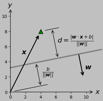
Several candidate methods exist to measure the distance \(d\) from a line to a point \(\boldsymbol{x}\). I chose to transform the line information into Hesse form \((\boldsymbol{w},\,b)\) and then evaluate \(d=(\boldsymbol{w}\cdot \boldsymbol{x}+b)/||\boldsymbol{w}||\):
(I ran into a bug where certain connecting lines sometimes pointed in the 180° wrong direction—specifically, when the slope of the main line was negative. I couldn’t find the error in my dot product or trigonometric calculations, so I just multiplied one of the distance parameters by the sign of the slope to ensure correct plotting, as commented in the code below. I still don’t know exactly where the problem lies.)
def get_line_distance_and_perp(line_slope, line_intercept, data_point):
	# transform line equation into Hess form
	(w1, w2, b) = (-line_slope, 1, -line_intercept)
	# apply the distance formula d = (w·x+b)/||w|| to get the distance
	# between where we are and where we want to be
	line_distance_diff = (np.array((w1, w2)) @ np.array(data_point)
		+ b) / np.linalg.norm((w1, w2))
	# also get the difference in slope between where we are
	# and where we want to be
	slope_angle_diff = np.arctan2(line_slope, 1)-np.arctan2(data_slope, 1)
	line_perp_slope = -1/line_slope
	line_perp_angle = np.arctan2(line_perp_slope, 1)
	# fix problem with the connecting lines sometimes pointing in the wrong direction
	line_distance_diff = line_distance_diff * line_slope / abs(line_slope)
	(line_point_x, line_point_y) = (data_point[0]
		+ line_distance_diff * np.cos(line_perp_angle),
		data_point[1] + line_distance_diff * np.sin(line_perp_angle))
	return line_distance_diff, slope_angle_diff, (line_point_x, line_point_y)
Then, we apply this function to get the original line distance and slope difference information relative to the center of mass of the data points:
(line_distance_diff, slope_angle_diff) = get_line_distance_and_perp(
	line_slope_0, line_intercept_0, (average_x, average_y))[0:2]
It’s this distance and slope that we’ll successively allow to oscillate. This brings us to a part of the code I’m obviously particularly excited about—the oscillation code. Again, we’re visualizing a mass \(m\) attached to a spring with spring constant \(k\) and a damper with viscosity \(c\) that’s pulled out of its equilibrium position and then allowed to retract.
def get_osc_funct(time): # set some values for pleasing oscillation
	k = 4 # spring value
	m = 1 # mass value
	c = 1.2 # damper value
	wn = np.sqrt(k / m) # natural frequency
	z = c / (2 * m * wn) # damping coefficient
	wd = np.sqrt(1 - z**2) * wn # damped natural frequency
	osc_funct = np.exp(-z * wn * time) * (np.cos(wd * time)
		+ z / np.sqrt(1 - z**2) * np.sin(wd * time))
	return osc_funct
We can now formulate a function that sends back the correct time-dependent intercept and slope depending on whether we’re translating (int) or twisting (slope):
def get_line(line_distance_diff, slope_angle_diff,
	data_point, time, parameter):
	# apply pleasing oscillation to either the distance or the slope
	if parameter == "int": # here, the distance oscillates;
	# return the appropriate fitting line slope and intercept
		line_distance = line_distance_diff * get_osc_funct(time)
		line_slope = line_slope_0
		line_perp_slope = -1 / line_slope_0
		line_perp_angle = np.arctan(line_perp_slope)
		(line_point_x, line_point_y) = (data_point[0]
			+ line_distance * np.cos(line_perp_angle),
			data_point[1] + line_distance * np.sin(line_perp_angle))
		line_intercept = line_point_y - line_slope_0 * line_point_x
	elif parameter == "slope": # here, the angle oscillates; again,
	# return the appropriate fitting line slope and intercept
		slope_angle_difference = slope_angle_diff * get_osc_funct(time)
		line_slope = np.tan(slope_angle_difference + np.arctan(data_slope))
		line_intercept = data_point[1] - line_slope * data_point[0]
	return line_slope, line_intercept
This is enough to achieve boinging in a line—either in its intercept or its slope.
It was a little harder to figure out the best way to make a polynomial twist into place. The approach I took—and this is just one of many possible strategies—is to take several vertical distances between the fitting line and the fitting polynomial (at 5 locations spread across the \(x\) axis, for example) and let those distances oscillate with our standard oscillation function. Then, a polynomial is fitted to these oscillating endpoints, and that polynomial is used as the dynamically changing polynomial. In practice, having the number of points be about 2 larger than the polynomial degree works fine, I think.
polynomial_spacing = polynomial_degree + 2 # makes polynomial oscillation smooth
poly_x_spaced = np.linspace(min_plot, max_plot, polynomial_spacing)
poly_distances = [data_poly_eval(a) - (a * data_slope
	+ data_intercept) for a in poly_x_spaced]
def get_polynomial(data_slope, data_intercept, poly_distances, time):
	trans_poly_distances = [x * (1 - get_osc_funct(time)) for x in poly_distances]
	trans_poly_x = [a for a, b in zip(poly_x_spaced, trans_poly_distances)]
	trans_poly_y = [data_slope * a + data_intercept + b
		for a, b in zip(poly_x_spaced, trans_poly_distances)]
	trans_poly_fit = np.polyfit(trans_poly_x, trans_poly_y, polynomial_degree)
	trans_poly_eval = np.poly1d(trans_poly_fit)
	return trans_poly_fit, trans_poly_eval
Here’s a visualization of those several vertical lines:
I wanted the thin red lines—er, the connecting lines—to continue to link the data points to the fitted function, but this aspect gets a bit more programmatically intricate when the function goes from being a line to a curve (essentially because several locations on a curve might be the same minimum distance from a particular point, which never happens with a line). My solution is to dive into the mathematical machinery of calculus, taking the derivative of the distance and setting that expression to zero.
def get_closest_point(poly_fit, poly_eval, data_point):
	xx = symbols("xx")
	list0 = np.ndarray.tolist(poly_fit)
	poly_fit_sym = Poly(list0, xx)
	# take the derivative of the fitted polynomial
	poly_deriv_sym = poly_fit_sym.diff(xx)
	# set the following term to zero to minimize the (square of the)
	# distance between the point and polynomial
	equation = xx - data_point[0] + (poly_fit_sym - data_point[1]) * poly_deriv_sym
	coeff = Poly(equation).all_coeffs()
	solved = np.roots(coeff)
	# chop any tiny imaginary component arising from the numerical solution
	solved = solved.real[abs(solved.imag) < 1e-6]
	dist = [(n - data_point[0])**2 + (data_poly_eval(n)
		- data_point[1])**2 for n in solved] # calculate distances from roots
	solved = solved[np.argmin(dist)] # get shortest distance if there’s more than one
	return solved, poly_eval(solved)
We now plot the fitting lines/curves (i.e., the line that twists into a polynomial). We actually need two of them, since one fades out as the other one fades in.
fit_line_color = ’0.5’
component_1_curve, = ax.plot((min_plot, max_plot),
	(min_plot * line_slope_0 + line_intercept_0, max_plot * line_slope_0
	+ line_intercept_0), lw = 3, color = fit_line_color, zorder = 0)
component_2_curve, = ax.plot((min_plot, max_plot),
	(min_plot * line_slope_0 + line_intercept_0, max_plot * line_slope_0
	+ line_intercept_0), lw = 3, color = fit_line_color, zorder = -2)
And then we make the thinner connecting lines and plot the actual points:
connector_line = []
for i in range(len(data_x)):
	(line_point_x, line_point_y) = get_line_distance_and_perp(line_slope_0,
		line_intercept_0, (data_x[i], data_y[i]))[2]
	connector_line_component, = ax.plot((data_x[i], line_point_x),
		(data_y[i], line_point_y),
		lw = 1, color = ’r’, zorder = -1)
	connector_line.append(connector_line_component)
ax.plot(data_x, data_y, marker = "o",
	markerfacecolor = ’red’, **marker_style, zorder = 0)
Now we get into the animation details, starting with frame rates and frame numbers. I wanted to ultimately get very smooth movement (which is slow to compile) with the option for fast compilation when trying out different settings, so I added a smoothness parameter to control the temporal resolution. I also defined the different scenes for the different motions and set their lengths in terms of frames. (I ended up not pausing at all between the steps of intercept_oscillation and slope_oscillation, and so the intercept_pause frame number is set as 0.)
smoothness = 1 # essentially a multiple of the frame rate;
# a setting of 1 is good for prototyping, and 5 is very smooth
frame_list = [[’fadein’, 6],
	[’fadein_pause’, 2],
	[’intercept_oscillate’, 8],
	[’intercept_pause’, 0],
	[’slope_oscillate’, 8],
	[’slope_pause’, 2],
	[’poly_oscillate’, 8],
	[’poly_pause’, 2],
	[’fadeout’, 6],
	[’fadeout_pause’, 2]]
It’s useful to define some frame-related parameters and some functions to get the very important times that govern movement and opacity.
frame_names = [i[0] for i in frame_list]
frame_durations = [smoothness * i[1] for i in frame_list]
def time_past(period): # total time before a certain segment
	return sum(frame_durations[0:frame_names.index(period)])
def time_future(period): # total time including a certain segment
	return sum(frame_durations[0:frame_names.index(period) + 1])
def time_present(period): # duration of a certain segment
	return frame_durations[frame_names.index(period)]
def norm_time(i, period): # how far we are into a certain segment
	return (i - time_past(period)) / time_present(period)
def effective_time(i, period): # used as the time in the oscillation function
	return (i - time_past(period)) / smoothness
Now for the big animation function. This function progresses through the scenes and applies the appropriate movement or opacity transition for each. The three adjustable features (component_1_curve, component_2_curve, and connector_line) are treated as objects whose coordinates and visual features can be adjusted as appropriate. All of the geometric line- and polynomial-fitting functions listed above are called to get the relevant coordinates.
When fading objects in and out with set_alpha, I often used min and max to ensure that the output would be bounded within 0 and 1, as required.
def init():
	return (component_1_curve, component_2_curve, connector_line,)
print("Starting to accumulate animation frames")
def update(i):
	print(f"Frame: {i+1}")
	if i == 0:
		component_2_curve.set_alpha(0) # the second line is set as invisible
		component_1_curve.set_alpha(1) # the first line is set as visible
		for j in range(len(data_x)): # set all the connector lines
			(line_point_x, line_point_y) = get_line_distance_and_perp(line_slope_0,
				line_intercept_0, (data_x[j], data_y[j]))[-1]
			connector_line[j].set_xdata((data_x[j], line_point_x))
			connector_line[j].set_ydata((data_y[j], line_point_y))
	if i <= time_future(’fadein’): # this is the component line fade-in part
		for j in range(len(data_x)): # the connector lines fade in
			connector_line[j].set_alpha(min(norm_time(i, ’fadein’), 1))
	elif i <= time_future(’fadein_pause’): # pause if desired
		pass
	elif i <= time_future(’intercept_oscillate’): # this the line translation part
		(line_slope, line_intercept) = get_line(line_distance_diff, slope_angle_diff,
			(average_x, average_y), effective_time(i,
			’intercept_oscillate’), "int")[0:2]
		component_1_curve.set_ydata((min_plot * line_slope + line_intercept,
			max_plot * line_slope + line_intercept))
		for j in range(len(data_x)):
			(line_point_x, line_point_y) = get_line_distance_and_perp(line_slope,
				line_intercept, (data_x[j], data_y[j]))[-1]
			connector_line[j].set_xdata((data_x[j], line_point_x))
			connector_line[j].set_ydata((data_y[j], line_point_y))
	elif i <= time_future(’intercept_pause’): # pause if desired
		pass
	elif i <= time_future(’slope_oscillate’): # this is the line rotation part
		(line_slope, line_intercept) = get_line(0,
			slope_angle_diff, (average_x, average_y),
			effective_time(i, ’slope_oscillate’), "slope")[0:2]
		component_1_curve.set_ydata((min_plot * line_slope + line_intercept,
			max_plot * line_slope + line_intercept))
		for j in range(len(data_x)):
			(line_point_x, line_point_y) = get_line_distance_and_perp(line_slope,
				line_intercept, (data_x[j], data_y[j]))[-1]
			connector_line[j].set_xdata((data_x[j], line_point_x))
			connector_line[j].set_ydata((data_y[j], line_point_y))
	elif i <= time_future(’slope_pause’): # pause if desired
		pass
	elif i <= time_future(’poly_oscillate’): # this is the polynomial part
		component_1_curve.set_xdata(x_spaced)
		(trans_poly_fit, trans_poly_eval) = get_polynomial(data_slope,
			data_intercept, poly_distances, effective_time(i, ’poly_oscillate’))
		component_1_curve.set_ydata(trans_poly_eval(x_spaced))
		for j in range(len(data_x)):
	 		(x_closest_point, y_closest_point) = get_closest_point(trans_poly_fit,
				trans_poly_eval, (data_x[j], data_y[j]))
	 		connector_line[j].set_xdata((data_x[j], x_closest_point))
	 		connector_line[j].set_ydata((data_y[j], y_closest_point))
	elif i <= time_future(’poly_pause’): # pause if desired
		pass
	elif i <= time_future(’fadeout’):
		# fade from the correctly fitted line to the original line
		# speed up the fade-out a little relative to the fade-in
		fade_speedup = 2
		for j in range(len(data_x)):
			connector_line[j].set_alpha(max(1
				- fade_speedup * norm_time(i, ’fadeout’), 0))
		component_1_curve.set_alpha(max(1 - fade_speedup * norm_time(i, ’fadeout’), 0))
		component_2_curve.set_alpha(min(norm_time(i, ’fadeout’), 1))
	elif i <= time_future(’fadeout_pause’): # pause if desired
		pass
	return (component_1_curve, component_2_curve, connector_line,)
Finally, the animation is implemented and the results saved using imagemagick. Note how the frame timing is adjusted using smoothness.
anim = FuncAnimation(fig, update, frames = sum(frame_durations),
	interval = 100 / smoothness, init_func = init, blit = False)
anim.save(’animation.gif’, dpi = 72, writer = ’imagemagick’)
print(’Done’)
One more example of the random selection, fitting, and oscillation:
Then, to get practice in writing object-oriented code, I rewrote the program to use classes for all the lines and animation.