Introduction
My parents bought me Richard Feynman’s (first) autobiography, Surely You’re Joking, Mr. Feynman! soon after it came out, around 1985. I remember being struck by one passage in particular:
I went to Princeton to do graduate work, and in the spring I went once again to the
Bell Labs in New York to apply for a summer job. I loved to tour the Bell Labs. Bill
Shockley, the guy who invented transistors, would show me around. I remember
somebody’s room where they had marked a window: The George Washington Bridge was
being built, and these guys in the lab were watching its progress. They had plotted the
original curve when the main cable was first put up, and they could measure the small
differences as the bridge was being suspended from it, as the curve turned into a
parabola. It was just the kind of thing I would like to be able to think of doing. I admired
those guys; I was always hoping I could work with them one day. [boldface emphasis mine]
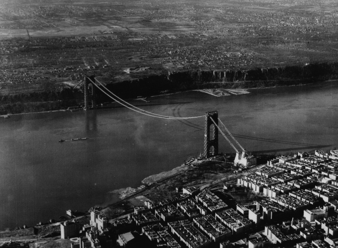
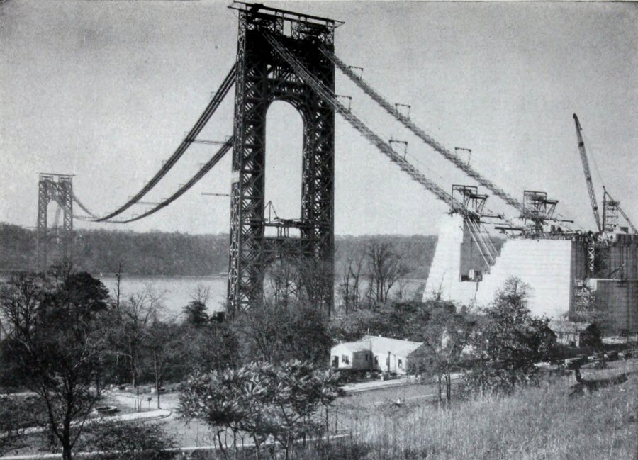
In situ assembly and installation of the four main cables during construction of the George Washington Bridge (courtesy Port Authority of New York and New Jersey).
At the time, I hadn’t heard of a catenary—the “original curve” Feynman refers to—but the description was memorable. What did these curves indicate, and why would one transition to the other?
The heated beam: Preliminaries & the case of axial conduction only
Later, when I was at graduate school at the University of Maryland, my advisor asked me to study microfabricated silicon actuators—tiny (mm-length) suspended beams that could push other objects around via thermal expansion from an applied current (as described here). Getting up to speed on the heat transfer analysis would have been a struggle had I not just taken Prof. Tim Shih’s heat transfer class.
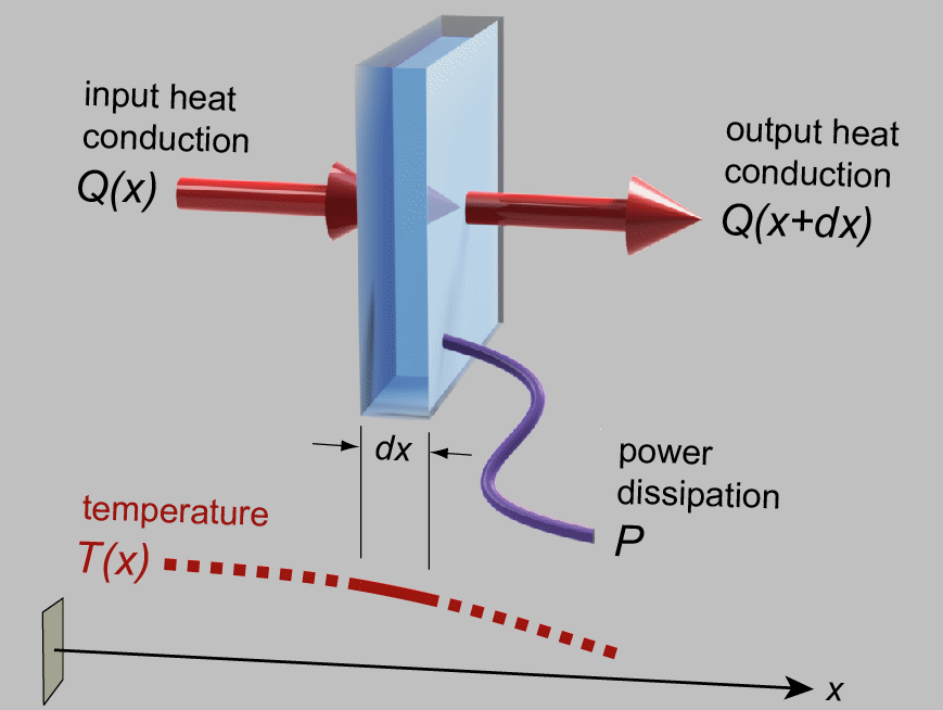
Shih spent a lot of time on energy balances. Shortly into the course, he started drawing a differential element on the blackboard at the beginning of each lecture with inputs and outputs, and he would sum the components. This energy-balance approach is quite far-reaching! Considering just the 1-D case, which is suitable for a long, narrow beam, we can designate the conductive heat rate \(Q\) (measured in watts in SI units) entering from the left at location \(x\) as $$Q(x)=-kA\frac{dT(x)}{dx},$$ corresponding to Fourier’s law of conduction, where \(k\) is the thermal conductivity, \(A\) is the cross-sectional area, \(T\) is the temperature, and \(x\) is the distance along the beam. (We’ll assume throughout this note that all material properties are constant.) That is, thermal energy tends to flow down a temperature gradient, mediated by the thermal conductivity of the material and the cross-sectional area. On the right side of the element, at \(x+dx\), the thermal energy exiting the element is generally a little different from that on the left side. We could simply write $$Q(x+dx)=-kA\frac{dT(x+dx)}{dx}$$ to incorporate this small difference. But since \(dx\) is small, let’s use a Taylor series expansion to approximate \(T(x+dx)\) as \(T(x)+\frac{d T(x)}{d x}dx\); thus, $$Q(x+dx)\approx-kA\frac{dT(x)}{dx}-kA\frac{d^2T(x)}{dx^2}dx.$$
(Such an approximation is exactly equivalent to saying that the differential element pictured above is so small that the temperature profile is nearly straight at that magnification.)
With an input heat rate of \(Q(x)\) and an output rate of \(Q(x+dx)\), it’s a matter of simple subtraction to find that we’re left with a contribution of \(kA\frac{d^2 T(x)}{dx^2}dx\) or, volumetrically, \(k\frac{d^2 T(x)}{dx^2}\), representing conduction in the resulting heat equation. And if thermal energy is generated in the beam at a volumetric power rate of \(P\), we might add a heat generation term to obtain a constitutive equation of $$k\frac{d^2 T(x)}{dx^2}+P=0,$$
where the sum of all input and output terms is zero at steady state. This equation can be expressed in words as follows: the degree to which the temperature profile curves downward is proportional to the amount of power being dissipated in the material.
Now, the first or second time I saw this approach in class, I thought, “Uhh… OK… Clearly this procedure is too intricate to be part of an exam; I’ll just memorize the final result.” But Shih kept drawing the schematic and reviewing the Taylor series expansion and summing the energy contributions in every single class. The fifth or sixth time, I thought, “Why is he wasting time going through this again?” When the tests asked us to draw the same schematic and derive the same result, I thought, “What’s the point?” Now, twenty years later, I’m still immediately able to perform an energy balance and a Taylor series expansion, those most valuable tools used to generate constitutive laws, and this ability was essential in analyzing a microfabricated device that actually did take the form of a narrow beam:
ANSYS simulation of the thermal heating and expansion and lateral deflection of a microfabricated beam. Note that I discuss only the beam’s temperature profile in this note, not its thermal-expansion-induced deflection, which forms neither a parabola nor a catenary. This deflection is calculated here.
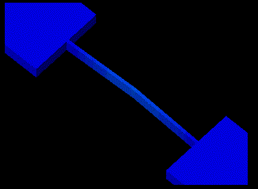
So when I started studying suspended silicon beams that heated up from an applied current (and in turn deformed from thermal expansion), it was straightforward to draw an energy balance with the volumetric conduction within the beam represented as \(k\frac{d^2 T(x)}{dx^2}\) and the heat generation represented as \(J^2\rho\), where \(J\) is the current density in the beam (i.e., the current per unit cross-sectional area) and \(\rho\) is the resistivity. (This is so-called Joule or resistive heating, which arises from electrons working their inefficient way through a material.)
The solution to the resulting energy balance equation,
$$k\frac{d^2T(x)}{dx^2}+J^2\rho=0,$$
is as simple as integrating twice, yielding
$$T(x)=-\frac{J^2\rho x^2}{2k}+C_1x+C_2,$$ and using the boundary conditions to determine the constants. Let’s assume that the beam of length \(L\) is centered at \(x=0\) and that the temperature is measured relative to the ambient temperature; with large blocks serving as ambient-temperature thermal reservoirs at either end of the beam, as shown above, we have $$T\left(-\frac{L}{2}\right)=T\left(\frac{L}{2}\right)=0,$$ and symmetry gives us $$T^\prime(0)=0$$ (here, I’m using the prime notation for a derivative with respect to \(x\)) so that $$T(x)=\frac{J^2\rho(L^2/4-x^2)}{2k}\propto C+x^2$$ where \(C\) is some constant. This is the equation for a parabola. Thus, the temperature distribution assumes a parabolic shape that starts at a relative increase of \(T=0\) at the anchors and increases to a maximum in the center.
The heated beam: Incorporating lateral heat transfer
Now let’s add a slight twist: in practice, with the microfabricated beams, there’s also a lateral energy departure term that’s dependent on the difference between the local and ambient temperature. (It’s not quite convection, although its form is convection-like. It’s the heat transfer to the adjacent substrate, which is as little as a micron or two away, as described here.) The resulting differential equation is $$k\frac{d^2T(x)}{dx^2}+J^2\rho-rT(x)=0,$$ where the parameter \(r\) captures information about that lateral heat transfer. Let’s solve this constitutive equation.
Laplace transforms are fantastic because they turn integrodifferential equations into algebraic equations, offering the potential for substantial simplification. A fun way to solve our equation is to take its Laplace transform,
$$\mathcal{L}\left[k\frac{d^2T(x)}{dx^2}+J^2\rho-rT(x)=0\right],\;\dots$$
Wait, no, that’s not going to be that much fun in the current state. Let’s simplify things by making the variable substitution \(\hat{T}(x)=T(x)-J^2\rho/r\) and dividing by \(k\), giving us the tighter
$$\mathcal{L}\left[\frac{d^2\hat{T}(x)}{dx^2}-\frac{r\hat{T}(x)}{k}=0\right].$$
OK, that’s much better. The Laplace transform of any function on its own, \(\mathcal{L}\left[\hat{T}(x)\right]\), is just \(\hat{T}(s)\), and any multiplicative constant carries through. In addition, the Laplace transform of a second derivative is
$$\mathcal{L}\left[\frac{d^2\hat{T}(x)}{dx^2}\right]=s^2\hat{T}(s)-s\hat{T}(0)-\hat{T}^\prime(0),$$
where \(\hat{T}(0)\) is the value of the function at point zero and \(\hat{T}^\prime(0)\) is the value of the first derivative at point zero. Since we’re taking \(x=0\) at the middle of the beam, by symmetry, we can say that the slope of the temperature distribution at that point is zero; thus, \(\hat{T}^\prime(0)=0\). This condition gives us
$$s^2\hat{T}(s)-s\hat{T}(0)-\frac{r\hat{T}(s)}{k}=0,$$
or, rearranging,
$$\hat{T}(s)=\frac{s\hat{T}(0)}{s^2-r/k}.$$
Since the inverse Laplace transform of \(s/(s^2-c^2)\) for any constant \(c\) is \(\cosh(cx)\), where \(\cosh\) is the hyperbolic cosine function, we find the solution to be
$$\hat{T}(x)=\hat{T}(0)\cosh \left(x\sqrt{\frac{r}{k}}\right)\propto\cosh(Cx).$$
This is the equation for a catenary. Huh—the temperature distribution itself has changed shape as a result of the presence of lateral heat transfer.
The complete equation, plugging in the boundary conditions, is
$$T(x)=\frac{J^2\rho}{r}\left(1-\frac{\cosh\left(x\sqrt{\frac{r}{k}}\right)}{\cosh\left(\frac{L}{2}\sqrt{\frac{r}{k}}\right)}\right).$$
Let’s check that this solution makes sense. The temperature scales linearly with the magnitude of resistive heating \(J^2\rho\). OK. The temperature increase is zero at either end of the beam. OK. If the lateral heat departure rate is infinite, then by \(T(x)\propto 1/r\), there’s no temperature increase (in this case, any thermal energy from resistive heating is swept away). OK. And if the thermal conductivity \(k\) is infinite, then there’s also no temperature increase because \(\cosh 0=1\) (in this case, the thermal energy is injected straight into the anchors). OK.
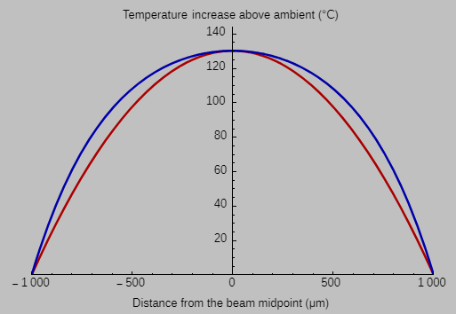
The two functions we’ve obtained (red for thermal conduction only, blue for the addition of lateral heat loss) are shown here for a 2-mm-long suspended silicon beam with an electrical resistivity of 0.001 Ω cm and a thermal conductivity of 150 W m-1K-1:
(You can create the same plot by entering the following Mathematica code:
With[{L = 2000, V = 1.25, rho = 10, k = 0.000150, r = (10^-18)10^9},
 Print[voltageIncreaseRatio =
  Sqrt[V^2/rho/L^2/2/k(L/2)^2/(V^2/rho/L^2/r (1-1/Cosh[L/2 Sqrt[r/k]]))]];
 Framed[Labeled[Plot[
  {V^2/rho/L^2/2/k ((L/2)^2-x^2),
  voltageIncreaseRatio^2 V^2/rho/L^2/r (1-Cosh[x Sqrt[r/k]]/Cosh[L/2 Sqrt[r/k]])},
  {x,-L/2,L/2},
  PlotRange->{{-L/2,L/2},{0,144}},
  PlotRangePadding->0,
  AxesOrigin->{0,0},
  ImageSize->{500, 300},
  DefaultTicksStyle->Black,
  Background->RGBColor["#C0C0C0"],
  PlotStyle->{Directive[Thickness[0.005], {Darker[Red]}],
  Directive[Thickness[0.005], {Darker[Blue]}]},
  AxesStyle->Directive[{Bottom, Top}, Black, FontFamily->"Arial", 13]],
  {"Distance from the beam midpoint (\[Micro]m)",
  "Temperature increase above ambient (\[Degree]C)"},
  {Bottom, Top},
  LabelStyle->Directive[Black, FontFamily->"Arial"]],
  Background->RGBColor["#C0C0C0"],
  FrameMargins->20]]
at Wolfram Cloud. Note that I’m working in microns in the code.)
The red curve shows the steady-state parabolic temperature distribution that arises when axial thermal conduction within the beam dominates; the applied voltage being simulated is 1.25 V. But if the beam is just a micron or two away from a large, flat, ambient-temperature substrate, then the lateral heat loss can be enormous—in this case, on the order of 109 W m-3. In this case, shown in blue, we have to nearly double the voltage across the beam to obtain the same maximum temperature. (This inefficiency motivates making the gap between the suspended beam and the substrate as large as possible in the fabrication process.)
The blue curve displays a catenary-like shape that’s somewhat flatter in the middle because far from the ends, the conduction to the large thermal reservoirs isn’t as important, whereas the lateral heat-transfer term acts throughout the beam. Relatively less axial conduction means a gentler axial temperature gradient.
The heated beam: And now a quick exercise
There’s not a much more fun-filled activity on a Friday night than examining interesting cases such as a small lateral heat departure term (representing only a slight degree of convection). We know that the parabolic temperature distribution must switch to a catenary-based curve for any finite convection-like term \(r\); how does this change occur?
The favored approach to investigating small deviations from an intricate expression is to apply the Taylor series expansion mentioned above. Put mathematically, for a small deviation \(\delta\) around some point \(z_0\) for a smooth function \(f(z)\), we have
$$f(z_0+\delta)=f(z_0)+f^\prime (z_0)\delta+\frac{1}{2!}f^{\prime\prime}(z_0)\delta^2+\frac{1}{3!}f^{\prime\prime\prime}(z_0)\delta^3+\frac{1}{4!}f^{\prime\prime\prime\prime}(z_0)\delta^4+\cdots$$
(Expressed in words, all that these additional terms do is refine our earlier notion that a curve observed close up looks nearly straight, OK, maybe with a slight quadratic curvature, OK, maybe with the tiniest additional cubic character, and so on.) From the earlier equation for the temperature distribution, we find the maximum temperature (i.e., at \(x=0\)) to be
$$T_\mathrm{max}=\frac{J^2\rho}{r}\left(1-\frac{1}{\cosh\left(\frac{L}{2}\sqrt{\frac{r}{k}}\right)}\right).$$
In fact, we need to go five terms deep in our Taylor series expansion before we find the first term of real interest. To see why this is the case, consider the successive derivatives of
$$f(z)=1-\frac{1}{\cosh (z)} $$
for small \(z=\frac{L}{2}\sqrt{\frac{r}{k}}\), and remember that \(\cosh 0=1\) and \(\sinh 0=0\):
$$f^\prime(z)= \frac{\sinh z}{\cosh^2 z}.$$ (This is just zero at \(z=0\).)
$$f^{\prime\prime} = \frac{1}{\cosh z}-\frac{2\sinh^2 z}{\cosh^3 z }.$$ (This is 1 at \(z=0\) and provides the parabola.)
$$f^{\prime\prime\prime} = -\frac{\sinh z}{\cosh^2 z}-\frac{4\sinh z}{\cosh^2 z}+\frac{6 \sinh^3 z}{\cosh^4 z}.$$ (Also zero at \(z=0\).)
$$f^{\prime\prime\prime\prime} = -\frac{5}{\cosh z}+\frac{28\sinh^2 z}{\cosh^3 z}-\frac{24\sinh^4 z}{\cosh^5 z}.$$ Aha! A term of \(-5\) appears, meaning that for small \(r\),
$$T_\mathrm{max}\approx\frac{J^2\rho}{r}\left(\frac{L^2r}{8k}-\frac{5L^4r^2}{384k^2}\right)=\frac{J^2L^2\rho}{8k}\left(1-\frac{5L^2r}{48k}\right).$$
So there we have it: as convection increases past a negligible amount, the original parabola (which represents heat transfer occurring through conduction alone) is slightly perturbed into a catenary-like expression with a temperature deviation of approximately \(5J^2\rho L^4r/384k^2\) at the hottest point.
The hanging chain: Preliminaries & the case of axial tension only
Let’s now switch to the example of a hanging chain (or cable, or string—these terms are all synonymous in this context). Here, the physics is substantially different: force balances and kinematics rather than energy balances and heat transfer. Our focus is now on the sag of the flexible chain rather than the temperature profile in a heated beam. How do the derivation and results differ?
Our strategy is now to balance forces in the plane of the hanging flexible line. The differential element appears as follows:
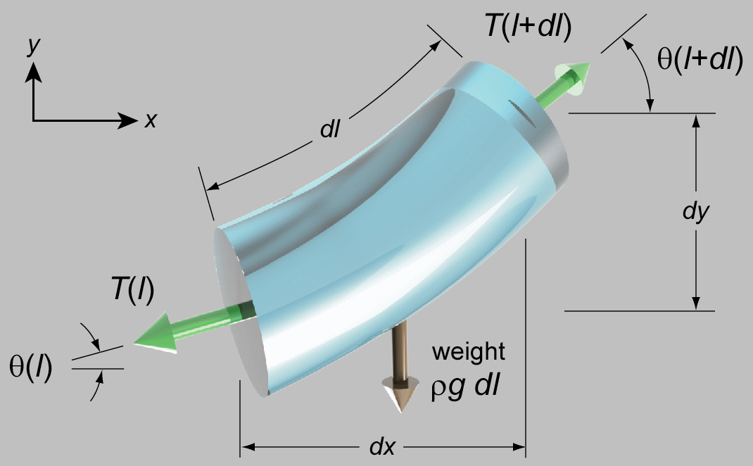
Here, \(T\) is now the tension, not the temperature, and \(\rho\) is now the mass per unit length of the hanging material, not the electrical resistivity of the beam; you’re responsible for distinguishing the difference. \(g\) is the acceleration from gravity, and \(l\) is the distance along the flexible line.
The most general case of a 3D differential element includes both forces (normal and shear) and moments applied to any arbitrary surface; however, the defining characteristic of the ideal flexible chain is that it cannot sustain a bending moment or shear. All you can do is pull on it. Therefore, only an axial tensile load appears in the diagram.
Unfortunately, although the heated beam yielded to an energy balance technique, I haven’t found a straightforward derivation of the shape of the chain using an analogous force balance. (Feynman might say that this is because I don’t understand the problem well enough.) The problem is that the tension within the chain changes from \(T(l)\) to \(T(l)+\frac{dT(l)}{dl}dl\) as the angle of the chain simultaneously changes from \(\theta(l)\) to \(\theta(l)+\frac{d\theta(l)}{dl}dl\). Thus, we end up with a surfeit of differential terms in the horizontal and vertical directions as we attempt to sum the resolved force components.
The standard way to work around this complication is to designate the tension at the lowest point of the chain as the constant \(T_0\):
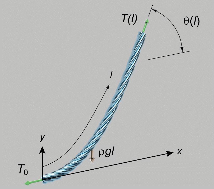
At any point on the chain, we can now perform a force balance in the \(x\) and \(y\) directions:
$$T\cos\theta=T_0$$ and
$$T\sin\theta=\rho g l.$$
Let’s divide the second equation by the first to obtain
$$\tan\theta=\frac{\rho g l}{T_0},$$ and let’s abbreviate \(\rho g/T_0\) as \(a\) for simplicity. This equation is interesting because by geometry, we also happen to have $$\frac{dy}{dx}=\tan\theta\,(=al),$$ and geometry also gives us $$dl^2=dx^2+dy^2.$$
Multiple derivations of the catenary equation appear online; here’s one such presentation. We start by differentiating \(dy/dx\) one more time with respect to \(x\), but in an interesting way:
$$\frac{d}{dx}\left(\frac{dy}{dx}\right)=\frac{d}{dl}\left(\frac{dy}{dx}\right)\frac{dl}{dx}=\frac{d}{dl}(al)\frac{d}{dx}\sqrt{dx^2+dy^2}=a\sqrt{1+\left(\frac{dy}{dx}\right)^2};$$ thus, $$y^{\prime\prime}=\frac{dy^\prime}{dx}=a\sqrt{1+\left(y^\prime\right)^2}.$$
(Again, I’m using the prime notation for a derivative with respect to \(x\).)
Now let’s separate variables and integrate once:
$$\int \frac{dy^\prime}{\sqrt{1+\left(y^\prime\right)^2}}=a\int dx;$$
$$\sinh^{-1} y^\prime=ax+C;$$
$$y^\prime=\sinh(ax+C).$$
As with the heated beam, we take the middle point, which by symmetry has a slope \(y^\prime\) of zero, to correspond to \(x=0\); thus, \(C=0\). We integrate again:
$$y(x)=\frac{1}{a}\cosh(ax)+C. $$
This is again the catenary equation, and the boundary conditions of \(y(\pm L/2)=0\) inform us that
$$y(x)=\frac{1}{a}\left[\cosh(ax)-\cosh\left(\frac{aL}{2}\right)\right].$$
The catenary profile of the completed footbridge of the George Washington Bridge (initially called the Hudson Bridge) (Skinner, “Roebling Cables for the Hudson River Bridge” (1930)).
Recall that no residual bending moment exists in the hanging chain at equilibrium; with no bending stiffness for a cable or chain, there couldn’t be. (Beams and rods, in contrast, can resist bending, by definition.) Thus, we have a calculation-free way to produce a corresponding stable arch with no bending moment simply by empirically tracing a hanging string and inverting the drawing to produce construction drawings for the arch. The ultimate limit to the slenderness of such an arch is buckling from imperfections or lateral loads (from the wind, for example).
Mechanics of materials textbooks often remark that Robert Hooke essentially founded the field of elasticity by publishing the phrase as goes the extension, so goes the force, translated into Latin and with the letters alphabetized—CEIINOSSSTTUU—to secure his priority until he published a more comprehensive treatment. (Nowadays, we might establish priority by publishing a cryptographic hash: 08076a66d18ff08d85e0d29a74f576ff49184e8c for that statement in English as processed by the SHA1 algorithm, for example.) Fewer engineers—but perhaps more architects—have heard that Hooke followed the same procedure for his solution for the catenary: as hangs the flexible line, so but inverted
stands the rigid arch (in Latin and alphabetized, ABCCCDDEEEEEFGGIIIIIIIILLMMMMNNNNNOOPRRSSSTTTTTTUUUUUUUUX; hashed, 6e23bdfd923ec5e8e198ec9afd9c59ae7f9d051f).
The hanging chain: Incorporating external loading
What if, as Feynman described, the chain or cable is ultimately loaded so substantially that its weight becomes insignificant relative to the load? This is generally the case with modern suspension bridges, for which the weight of the roadway is far larger than that of the cable. In this case, we can write the vertical component of the load in the diagram above as
$$T\sin\theta=wx,$$
where \(w\) is the weight of the distributed load per unit length. (The earlier cable self-weight term of \(\rho gl\) is now comparatively negligible.) Following the approach described above, we now have \(\tan\theta=dy/dx=wx/T_0\), which we can integrate and insert boundary conditions into to find that $$y=\frac{w}{2T_0}\left(x^2-\frac{L^2}{4}\right)\propto x^2+C,$$
which is of course a parabola. What a difference the switch from \(l\) to \(x\) makes in terms of ease of solution!
Feynman, Bell Labs, and the George Washington Bridge
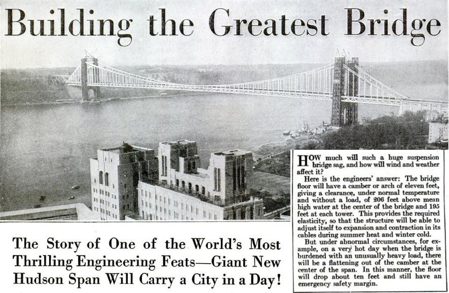
 Let’s consider the shapes that Feynman might have seen traced on the window at Bell Labs at 463 West Street in Manhattan, nine miles south of the bridge. First of all, when was this visit? Feynman reported visiting the site in the spring after his first year as a graduate student at Princeton, which would have been 1940. The bridge opened in 1931, and no further construction work is reported until 1946, when two more lanes were added to the upper deck (at the time, the only deck). So perhaps Feynman had spotted markings dating back to when the bridge was first constructed, about ten years earlier. Let’s consider the shapes that Feynman might have seen traced on the window at Bell Labs at 463 West Street in Manhattan, nine miles south of the bridge. First of all, when was this visit? Feynman reported visiting the site in the spring after his first year as a graduate student at Princeton, which would have been 1940. The bridge opened in 1931, and no further construction work is reported until 1946, when two more lanes were added to the upper deck (at the time, the only deck). So perhaps Feynman had spotted markings dating back to when the bridge was first constructed, about ten years earlier.
In any case, the main span of the George Washington Bridge measures 3500 ft, and the cable sag is approximately 325 ft. Let’s start by assuming the cable is inextensional, i.e., that it doesn’t stretch upon being loaded by its own weight or that of the roadway. We can estimate the necessary length of the cable for both the parabolic and catenary curves using the equation
$$l=2\int_0^{L/2}\sqrt{1+(y^\prime)^2}\,dx.$$
Maybe we’ve done enough analytical derivations at this point; let’s just numerically integrate this expression. The associated Wolfram Cloud commands are
lengthIntegrand[F_]:=Sqrt[1+D[F,x]^2];
With[{sag = -325., L2 = 3500/2},
 yParabola = sag(1-x^2/L2^2);
 length = NIntegrate[2lengthIntegrand[yParabola],{x,0,L2}]]
We find that the cable length is 3578.9 ft. Now let’s find the sag resulting from the same length of cable in catenary shape, subject to its own weight alone, before the weight of the roadway distorted it into a parabola:
Assuming[a > 0, With[{L2 = 3500/2},
 yCatenary = 1/a(Cosh[a x]-Cosh[a L2]);
 aSolution = NSolve[length == 2Integrate[lengthIntegrand[yCatenary],{x,0,L2}]&&a>0,a,Reals];
 yCatenary/.aSolution/.{x->0}]]
The sag of the catenary is 324.3 ft—a difference of only 8 inches! Let’s plot the two curves:
With[{sag = -325, L2 = 3500/2},
 Framed[Labeled[
  Plot[{yParabola,yCatenary/.aSolution},{x,-L2,L2},PlotRange->{{-L2,L2},{0,1.1sag}},
   AspectRatio->Automatic,PlotRangePadding->0,AxesOrigin->{0,0},
   ImageSize->{640,90},
   Ticks->{{-1500,-1000,-500,500,1000,1500},{-100,-200,-300}},
   Background->RGBColor["#C0C0C0"] ,
   PlotStyle->{Directive[Thickness[0.001],{Darker[Red]}],Directive[Thickness[0.001],{Darker[Blue]}]},
   AxesStyle->Directive[{Bottom,Top},Black,FontFamily->"Arial",13]],
  {"Sag relative to the connection points (ft)","Distance from the span midpoint (ft)"},
  {Bottom,Top},LabelStyle->Directive[Black,FontFamily->"Arial"]],
 Background->RGBColor["#C0C0C0"],FrameMargins->5]]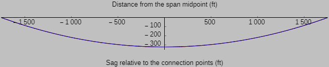
Notably, even with a reduced line width in the plot, the difference is almost indistinguishable between the catenary (shown in blue), representing the case of the cable weight alone, and the parabola (shown in red), representing the case of the hanging bridge weight far exceeding the cable weight. The similarity is precisely due to the fact that \((y^\prime)^2\) is quite small in the equations above for a sag-to-span ratio of less than 1:10, which is the case here.
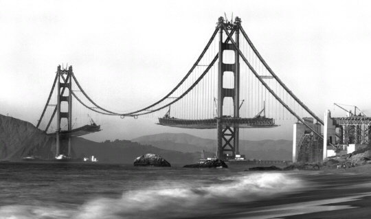 The staff at Bell Labs would have had to have sharp eyes indeed to distinguish these curves suitably using markings on a window from nine miles away. So what’s gone wrong in our analysis? One possible resolution is to return to the assumption of inextensibility. In fact, the cable does stretch, and bridges are built with an upward camber to accommodate this stretching, as shown in the construction photograph of the Golden Gate Bridge at left (courtesy Time Magazine). Therefore, I suspect that the difference Feynman described seeing at Bell Labs is not simply the transformation of a catenary to a parabola (for a set cable length); it was the transformation to a parabola plus substantial stretching of the cable. The staff at Bell Labs would have had to have sharp eyes indeed to distinguish these curves suitably using markings on a window from nine miles away. So what’s gone wrong in our analysis? One possible resolution is to return to the assumption of inextensibility. In fact, the cable does stretch, and bridges are built with an upward camber to accommodate this stretching, as shown in the construction photograph of the Golden Gate Bridge at left (courtesy Time Magazine). Therefore, I suspect that the difference Feynman described seeing at Bell Labs is not simply the transformation of a catenary to a parabola (for a set cable length); it was the transformation to a parabola plus substantial stretching of the cable.
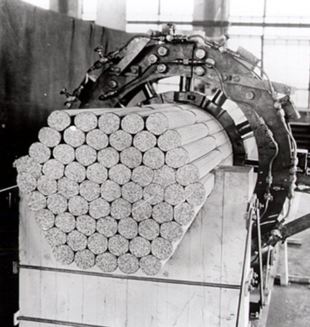 We can test this hypothesis by calculating the stretch of the cable due to its self-weight and the additional weight of the roadway. Four cables were used, each with 26,474 strands of 0.196-in-diameter high-carbon-steel wire (Young’s elastic modulus \(E\): about 30,000 ksi), as shown at right (courtesy Port Authority of New York and New Jersey). That much steel alone—a three-foot-diameter’s worth—weighs an astonishing 2700 lbs per linear cable foot, roughly the same as a Honda Civic; the addition of spaced shoes, wraps, and other hardware brings the weight to 3400 lbs/ft. We can test this hypothesis by calculating the stretch of the cable due to its self-weight and the additional weight of the roadway. Four cables were used, each with 26,474 strands of 0.196-in-diameter high-carbon-steel wire (Young’s elastic modulus \(E\): about 30,000 ksi), as shown at right (courtesy Port Authority of New York and New Jersey). That much steel alone—a three-foot-diameter’s worth—weighs an astonishing 2700 lbs per linear cable foot, roughly the same as a Honda Civic; the addition of spaced shoes, wraps, and other hardware brings the weight to 3400 lbs/ft.
I won’t bother with the equations for highly elastic catenaries, which incorporate nonuniform changes in density due to large stretching and are much more complex that those derived above. After all, the anticipated axial strain (i.e., the elongation per unit length) is very small, on the order of 0.1%. It’s sufficient to calculate the axial stress in the cable from the location-dependent tension and divide it by the stiffness to obtain the strain. As derived above, the tension in the catenary is \(T_\mathrm{catenary}(l)=\sqrt{T_{0,\mathrm{catenary}}^2+(\rho g l)^2}\), where \(T_{0,\mathrm{catenary}}=\rho g/a\) and where \(a\) can be found from the boundary conditions (namely, the span and sag); the tension in the parabola is \(T_\mathrm{parabola}(x)=\sqrt{T_{0,\mathrm{parabola}}^2+(wx)^2}\), where \(T_{0,\mathrm{parabola}}\) can also be found from the boundary conditions. The estimated dead load \(w(x)\) is 39,000 pounds per horizontal foot of roadway, divided over the four cables.
I find the tension in the cable alone to be approximately 16-17 million pounds (!) (depending on whether we’re looking at the point of maximum sag or the top point of attachment to the tower) and the tension in the cable from the dead load alone to be approximately 45-49 million pounds. The total tension matches the often-quoted value of 62 million pounds per cable, so we seem to be on the right track. And this much tension would correspond to a strain of \(T/(AE)\) or about 0.0026, or 14 feet in a cable 5300 ft long (now taking the total distance from abutment to abutment instead of from tower to tower), or about 30 feet of additional sag, of which about 7 corresponds to stretching from the cable self-weight.
Therefore, working backward, we find that the original sag before the roadway was installed must have been noticeably less than the final sag of 325 ft because of the axial stretching of the cable:
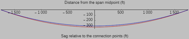
These results support the hypothesis that it was cable stretching, not just a change in shape from a catenary to a parabola, that was the most prominent change that the Bell Labs staff observed, as admired by Feynman. Fully loaded with cars and trucks (i.e., with an additional live load of 9,000 pounds/ft) and on a hot day, the roadway surface was predicted to move down at least an additional ten feet (see inset in the following):
This 1929 article shows a composite photograph and illustration; the bridge (other than the under-construction towers) is drawn in and is drawn as it would appear much later—the lower deck wasn’t even added until the 1960s (Ketchum, Scientific American (1929)).
In The George Washington Bridge: Poetry in Steel (2008), Rockland notes that when the lower deck was added in 1962, the suspender cables between the main cables and the roadway had to be adjusted to remove the additional sag from the new weight. Anticipating the eventual addition of a second level, the bridge’s designer, Othmar Ammann, had incorporated tie points on the suspender cables to accommodate this need. Indeed, the doubling of the cables to two per side in the original design was done specifically to allow a lower deck to be added at some later time. Even now, the George Washington Bridge remains “unfinished”—the two middle lanes in the lower deck are still unpaved.
Venturing into the time-dependent case
So we’ve seen that both heated beams and hanging chains transition between catenary-like and parabolic profiles depending on the loading conditions. Do these similarities continue if we look at the dynamic behavior? In fact they do not, and the constrasting results provide an excellent comparison between energy transport in the form of diffusion and energy transport in the form of a wave.
If the heated beam is not at steady state, then any excess energy goes into heating the differential element, and we must incorporate the time dependence of temperature by adding a term to the right side of the heat equation:
$$k\frac{\partial^2T(x,t)}{\partial x^2}+J^2\rho=\frac{k}{\alpha}\left(\frac{\partial T(x,t)}{\partial t}\right),$$
where \(\alpha\) is the thermal diffusivity and where the ordinary derivatives have turned into partial derivatives because the temperature is now a function of both position and time.
(The thermal diffusivity governs how quickly changes in temperature propagate over a distance. Because the thermal diffusivity of all solid food is similar to that of water, about 9 mm2 min-1, it always takes about 5 minutes per side—estimated using the approximate relationship of time = distance2/diffusivity—to pan-cook any half-inch-thick foodstuff, be it meat, fish, or vegetable.)
I discuss the solution to this time-dependent equation here, and we published that work here.
Now, if we look at the non-steady-state case of the hanging chain, we find that any unbalanced force must induce an acceleration, again appearing on the right side of the differential equation:
$$-\mathbf{T}(\mathbf{x},t)+\mathbf{T}(\mathbf{x}+d\mathbf{x},t)-\rho g\mathbf{k}\,dl=\rho \frac{d^2 \mathbf{x}(t)}{d t^2}\,dl,$$
where I’ve shifted to boldface for the tension \(\mathbf{T}\) and position \(\mathbf{x}\) vectors and the unit vector \(\mathbf{k}\) in the z direction. I won’t try to solve this equation here; the substantial increase in complexity relative to the time-dependent temperature equation is why transient behavior is covered in a few weeks in a heat transfer class but vibration of continuous media typically demands its own graduate course.
The difference between the implications of the first time derivative and the second time derivative on the right side of these equations is tremendous! For example:
The first time derivative describes diffusion behavior, in which there’s no well-defined speed and no inertia. That is, for standard systems (e.g., no combustion or other weird stuff), if we change the temperature somewhere, the propagating change will never overshoot our applied value. Diffusion processes occur through random motion and are undirected.
The second time derivative describes wave behavior. Waves do have a well-defined speed (related to the mass and restoring force), and mechanical waves do rely on inertia and commonly exhibit overshoot and reflection.
What is left?
How interesting this connection is between a heated bar and a hanging chain. After Hooke, we could remark that as hangs the flexible loaded line, so radiates the heated beam (ut pendet continuum flexile onustum, sic radiabit talea caloratum, AAAAAABCCCDDEEEEEFIIIIILLLLMMMNNNNOOOPRRSSTTTTTTTUUUUUUX, 81c8efac0dcec451d85a4e3f360e7539fcaa6ba8). Consider these aspects: - In each case, we have an axial element—thermal conduction and tension—and a corresponding clamped condition at the ends in terms of the temperature and position, respectively. In each case, we also have the potential for an additional load: a convective (or convection-like) term for the thermal beam and a distributed weight for the mechanical chain.
But the most convenient solution methods can be quite different. Would you have guessed from the two governing equations, namely, $$\hat{T}^{\prime\prime}=C\hat{T}$$ and $$y^{\prime\prime}=D\sqrt{1+\left(y^\prime\right)^2}$$ (where the constants \(C\) and \(D\) describe the key features of the corresponding system), that the hyperbolic cosine would emerge as a solution for each? Notably, the maximum temperature of the heated beam scales with the injected power; in fact, as the current density \(J\) increases, the temperature excursion increases as \(J^2\). In contrast, the maximum sag of the chain or cable doesn’t scale with gravity. Rather, the maximum sag remains nearly constant when we assume that the constitutive material is inextensional. Using the powerful framework of the energy or tension balance, one can investigate various other interesting problems. What if a substantial amount of heat from the beam is dissipated through radiation, for example, which scales with \(T^4\), as in the case of an incandescent filament? What if the string of interest is a spinning jump rope, in which the lateral loading scales as \(\omega^2 y\), where \(\omega\) is the rotational frequency? Substantial distributed external loading on the chain or cable transforms the catenary into a parabola; in contrast, distributed lateral heat loss in the heat-dissipating beam transforms a parabolic temperature distribution into a catenary-like profile. Can you resolve how this asymmetry arises?
|