• Measurements and modeling of the stiffness of a microscale tensioned membrane over a large temperature range (Storch et al., “Young’s modulus and thermal expansion of tensioned graphene membranes” Physical Review B (2018)).

• Resting steel spheres on thin compliant layers and laterally observing the deformation to characterize the film stiffness (Gross et al., “Simultaneous measurement of the Young’s modulus and the Poisson ratio of thin elastic layers” Soft Matter (2017)).

• Using speckle patterns and machine vision to characterize ceramic stiffness from deflection under a three-point bending test (Farsi et al., “Full deflection profile calculation and Young’s modulus optimisation for engineered high performance materials” Scientific Reports (2017)).

• Determining the bulk stiffness of a composite material containing unusually shaped nanoparticles embedded within a block copolymer matrix (Raja et al., “Influence of three-dimensional nanoparticle branching on the Young’s modulus of nanocomposites” PNAS (2015)).

Young’s modulus is so widely used that I’ll sometimes see an article refer to “the elastic modulus” (meaning Young’s elastic modulus) as if there’s only one:

• “Fiber diameter and orientation along with polymeric composition are the major factors that determine the elastic modulus of electrospun nano- and microfibers” Vatankhah et al. Acta Biomaterialia 10(2) (2014).

• “The elastic modulus of multilayer graphene is found to be more robust to damage created by high-energy α-particle irradiation as compared to monolayer graphene” Liu et al. Advanced Materials 27(43) (2015).

• “Our previous study showed that embryonic tendon elastic modulus increases as a function of developmental stage” Schiele et al. Journal of Orthopaedic Research 33(6) (2015).

and so on. Sometimes the meaning of the specific elastic modulus is clear from the context (or is later clarified), sometimes not.

But anyone interested in mechanics of materials or material physics needs to know about other elastic moduli (at a minimum, the shear modulus and the bulk modulus, as addressed in this note) to understand the origin, nature, and implications of elasticity in materials.

So let’s not overrate Young’s modulus; instead, let’s appreciate its advantages while understanding its limitations and what insights come with a familiarity with other types of stiffness.

From this discussion, and as the culmination of this note, derived below, we’ll obtain the equation

$$\epsilon_{ij}=\frac{1}{2G}\sigma_{ij}-\left(\frac{1}{6G}-\frac{1}{9K}\right)\delta_{ij}\sigma_{kk},$$

which powerfully describes, using contracted notation, the strain \(\epsilon\) resulting from any stress \(\sigma\) in any isotropic material deforming linearly and elastically. The essential material properties here are the shear modulus \(G\) and the bulk modulus \(K\), to be discussed in detail below. Notably, Young’s modulus doesn’t appear at all in this expression! The reason, as we’ll discover, is that Young’s modulus can be decomposed into other moduli that are arguably more fundamental in the context of general 3D deformation of materials.

The 1D framework

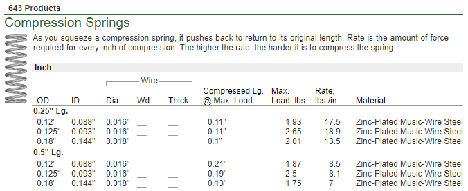
To get started, recall that an elastic modulus, in general, describes the relationship between a stress (i.e., a force applied per unit area) and a strain (i.e., a deformation normalized to an original distance). An elastic modulus, as a material property, is useful because to a certain degree it’s situation and geometry independent: an idealized spring can be cut in half, for example, to obtain two springs with the exact same elastic moduli, as the material is unchanged, but double the spring constant (that is, the halves are twice as stiff because there’s less spring to extend). In the McMaster-Carr catalog, for example, we can verify that real quarter-inch-long springs have approximately double the specified spring constant (“rate”) of the half-inch-long springs:

Elastic moduli are also generally useful because we wish to understand how a solid pulls or pushes back in response to (suitably small) forces. (At large forces, the predominant mechanism or the geometry may change; this the realm of nonlinear elasticity. Alternatively, the sample may not recover; this is the realm of plasticity.) And the elastic moduli are correlated in interesting ways to other material properties such as the melting temperature, density, heat capacity, and thermal expansion, providing insight into material physics.

Young’s modulus is arguably the preeminent elastic modulus (and thus a candidate for being overrated). It couples, very specifically, the axial stress and axial strain of a rod or bar subject to axial loads only. (There’s no distinction between a rod and a bar in this context; the criterion is only that the geometry is long and narrow. This condition ensures that every point in the sample is close to the stress-free surface; thus, no lateral stresses exist.) Those axial qualifiers tell us that this stress-strain relationship is a very 1D type of relationship (albeit including beam bending, which still relies on axial elongation and contraction). As a result, naive applications of Young’s modulus to other configurations—such as short bars, plates, thin films, or pressure vessels—are likely to be incorrect to a certain degree.

Under the 1D framework, we might apply a tensile or a compressive force \(F\) to the ends of a long, narrow object (let’s call it a rod) with cross-sectional area \(A\). The dogbone sample, for example, allows a firm grip while clearly defining the region to be stretched, and Young’s modulus is ideal for expressing its uniaxial elastic behavior:

Aluminum dogbone specimens manufactured for tensile testing (Pasco).

The resulting axial stress \(\sigma\) in the rod is \(\sigma=F/A\). The constitutive equation that quantifies the stress–strain coupling is simple Hooke’s Law:

$$\sigma=E\epsilon,$$

where \(E\) is Young’s modulus and \(\epsilon\) is the engineering strain, or normalized deformation, or finite elongation per unit length: \(\epsilon=\Delta L/L\). (I discuss a different definition of strain here.)

So this method offers a straightforward way to measure material stiffness in a 1D context. Fair enough. To understand why an elastic modulus other than Young’s modulus would ever be needed, we need to incorporate additional dimensions.

The 2D framework

Real objects exist in 3D, of course, but it’s instructive to consider a 2D case first to define a new set of terms and to appreciate the differences that arise when we extend our thinking to an arbitrary 3D chunk of material.

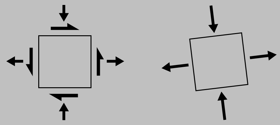
Let’s first draw a square in a fixed location and orientation in 2D and consider how it might be deformed. Specifically, let’s distinguish loads that tend to distort the square into a smaller or larger square or a rectangle (normal loads, those that come in from the sides and top and bottom and are perpendicular to the faces) from loads that tend to distort the square into a rhombus or diamond (shear loads, which act tangentially to the faces):

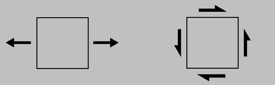
One can load the side of a fixed 2D square in two different ways: perpendicular or parallel to the side. The former requires a partner load on the opposite side to keep the square from accelerating away. The latter requires four (!) equal-strength components to keep the square from translating or rotating.

These two types of loads represent a dichotomy; they’re fundamentally different and produce different outcomes. When applied to a 2D square, we obtain the following distinct results: normal loads cause changes in side lengths, whereas shear loads cause changes in corner angles:

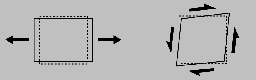
Typical deformation resulting from normal and shear loading.

(The normal loading case is drawn to incorporate the Poisson effect, or the lateral strain that generally occurs when one stretches or compresses a material. This relationship is mediated by Poisson’s ratio \(\nu\), which normalizes the lateral contractile strain relative to the axial elongational strain: \(\nu=-\frac{\epsilon_y}{\epsilon_x}\). Poisson’s ratio is typically positive; that is, we generally observe lateral contraction when we stretch a material.)

Right away, we encounter a new type of deformation (namely, shear) that requires us to now distinguish our elastic moduli:

• Young’s modulus mediates how much the side length of the square changes in the direction we pull (as an extension of the relationship of uniaxial stress vs. uniaxial strain described earlier). If the normal loading is applied along more than one axis, then we need to consider how the side length responds to the corresponding Poisson effect.

• The shear modulus mediates how much the corner angle changes as a result of a shear load.

Since there’s no guarantee that an arbitrary load would have entirely normal or entirely shear character, a whole segment of elasticity theory has arisen to interpret loads of intermediate character (the most well-known approach is Mohr’s circle, which provides a geometrical interpretation). In fact, any arbitrary loading state can be decomposed into a set of orthogonal (meaning mutually perpendicular) normal loads:

An arbitrary collection of normal and shear loads can always be decomposed into a set of solely normal stresses (the so-called principal stresses, which happen to be the eigenvalues of the stress matrix) if one allows the 2D element to be rotated.

Importantly, the transformation requires a change in orientation. As we proceed to considering real 3D objects, we immediately see that this ambiguity in orientation presents a problem with the classification of normal vs. shear loads.

The 3D framework

The dichotomy of normal vs. shear stresses for infinitesimal elements can’t be extended in general to real objects; here’s why. Consider a material undergoing uniaxial loading, and let’s position our 2D element in the middle of the material as shown below:

We can always draw a reference element on any object to be deformed. Images based on a photograph by Nielson Fitness.

Following the reasoning above, we’d interpret the axial load as exerting a normal stress on the element, thus elongating its side lengths. No problem, right? Such configurations are well handled using Young’s elastic modulus (with Poisson’s ratio describing the lateral strain):

But consider: If we simply rotated our conceptual element by 45°, we’d see an entirely different stress state. We’d see some degree of normal stress, but we’d also see substantial shear stress that would distort our original square into a diamond:

We encounter a paradox regarding whether either normal or shear deformations are being induced within the material. After all, Nature has no preferred orientation, so the appearance of different results for our different rotations becomes problematic. We’re left to conclude that we can’t generally transfer a certain loading configuration on an object to an arbitrary internal element in the material. This is the reason that the division of normal vs. shear stress and strain runs into problems in real materials (although these notions are totally appropriate for a well-defined surface because a surface has a built-in orientation).

Since we’re now thinking in 3D, let’s consider a stress state that acts on all three directions equally—and of course a familiar example is compressive equitriaxial stress, also known as hydrostatic stress, also known as pressure. A modulus describing a material’s resistance to a change in volume from a uniform application of pressure would be useful. This new modulus, the bulk modulus, truly brings us into the 3D realm. Now we have three types of elastic moduli:

• Young’s modulus mediates certain changes in a length.

• The shear modulus mediates certain changes in an angle.

• The bulk modulus mediates changes in the volume.

And we have a new dichotomy, as there are two ways to deform any 3D object: we could change its size or we could change its shape. The loading that changes an object’s size is known as dilatational stress. (The compressive version is pressure.) The loading that changes an object’s shape is known as deviatoric stress. (Think of this as a sort of 3D version of shear, although it doesn’t necessarily consist of shear loads.) These two different stress states are distinct, and one or the other or both arise in the response of any real material—be it solid, liquid, or gas—to a mechanical load.

Notably, the uniaxial loading state that’s so useful in measuring Young’s modulus produces a mix of internal dilatational and deviatoric stress states, making this loading type—and Young’s modulus—slightly… unsatisfying for considering the general loading of 3D objects. (This is the key point of this note.) As far back as 1856, William Thomson, later known as Lord Kelvin, identified the shear and bulk moduli as the two (and only two) so-called principal stiffnesses of an isotropic material ("Elements of a mathematical theory of elasticity, Part 1, On stresses and strains," Philosophical Transactions of the Royal Society 146, 481–498). These days, we call these two moduli the eigenstiffnesses or eigenelastic constants.

It turns out that the fundamentally different responses to deviatoric and dilatational loads provide substantial insight into material differences and practical use, including the potential for material failure under a load. Consider these values and correlations for various types of matter:

Features of the shear modulus

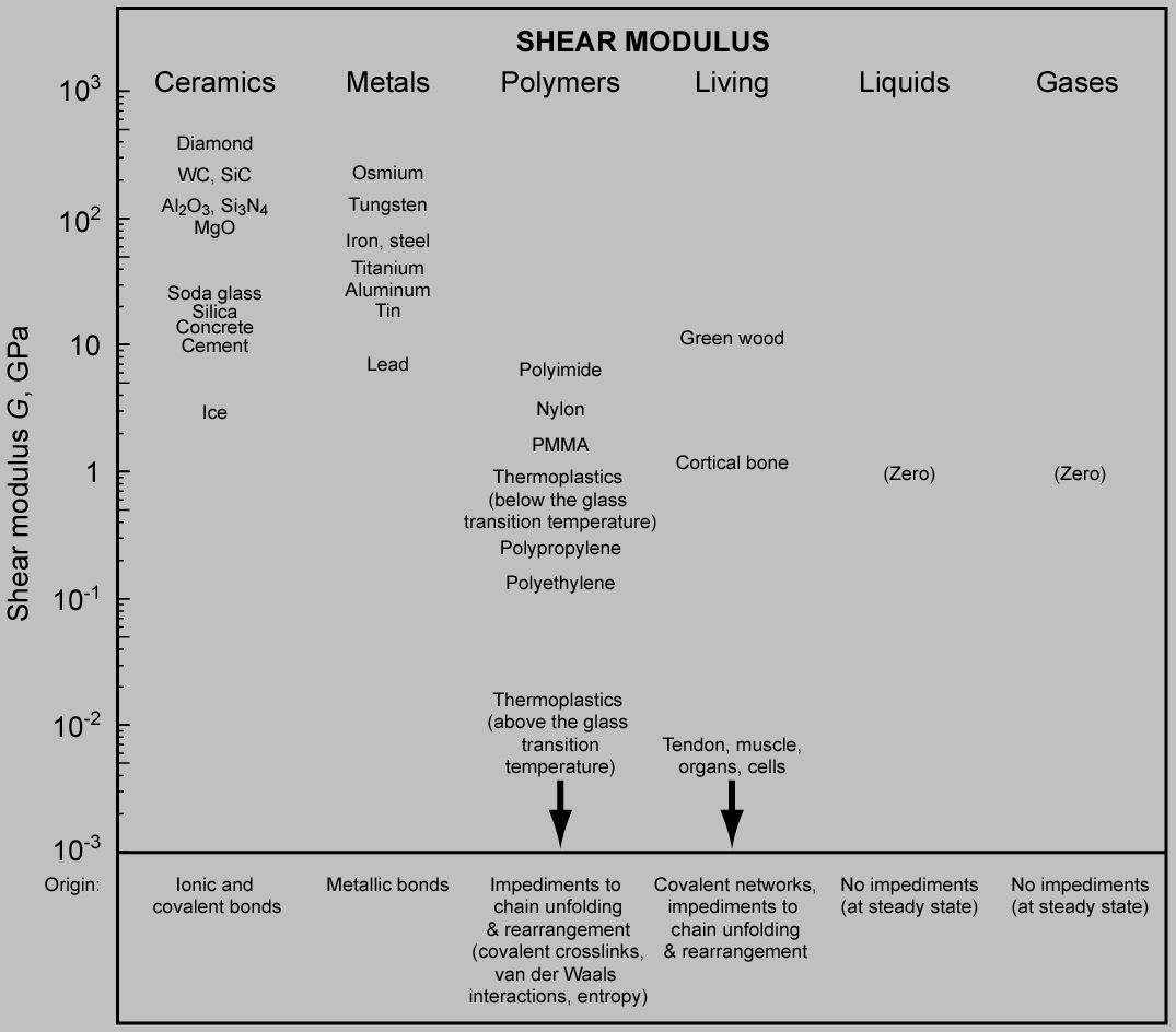
Approximate shear moduli of a variety of material types and the corresponding origins. The bonds in solids generally resist rearrangement. Notably, however, the chain bonding in polymers and some biological tissue allows substantial rearrangement (depending on the degree of crosslinking; minimally crosslinked elastomers such as rubber are particularly compliant in shear). Moreover, fluids (liquids and gases) shear effortlessly as the strain rate drops to zero.

The shear modulus is amazing! It’s got some neat properties:

• The shear modulus governs resistance to molecular rearrangement (as opposed to the bulk modulus, which governs resistance to changes in molecular spacing). Solids can sustain a deviatoric load over human timescales, meaning that they resist rearrangement, whereas simple fluids such as idealized liquids and gases cannot. As a result, it works as a first pass to assume that fluids have zero shear modulus (and zero Young’s modulus). Fluids simply don’t exhibit the relatively strong long-scale arrangements of intermolecular bonds that resist shear rearrangement in solids.

• Another key aspect: Shear is what causes every ductile material to fail. This aspect is important because ductile materials are essential in engineering practice—they tend to fail slowly and with accumulating evidence, as opposed to brittle materials that fail with little warning.

  Shear is a convenient way of coming apart under excessive loading because it’s so easy! Shear doesn’t require the creation of a new large surface (as cracking does), which costs substantial energy. Shear doesn’t even require an entire plane of atoms to shift at once. Instead, the shear we observe in real ductile materials occurs through dislocation glide, or the movement of 1D defects, which involves rows of atoms slipping past each other.

  
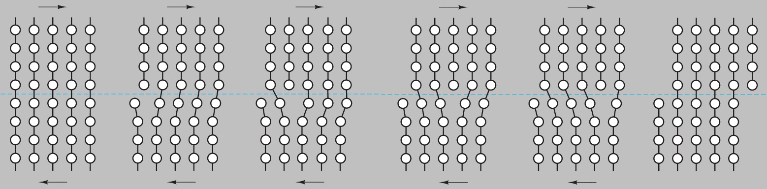
  Shear-induced plasticity, or permanent deformation, via edge dislocation glide in an idealized crystal. A 1D defect perpendicular to the page carries a slip step through the sample. Adapted from Shackelford’s Introduction to Materials Science for Engineers (Pearson 2015).

  This mechanism has been compared to moving a carpet by kicking a hump down its length or to the way a caterpillar moves by elongating one section at a time.

  So it doesn’t matter that uniaxial stretching with a dogbone specimen is a convenient experimental framework; shear (or the more sophisticated version, deviatoric stress) is the most important factor regarding failure in a ductile engineering material. Even when uniaxial tension is applied to a ductile dogbone specimen, the resulting plastic deformation is driven by shear stress.

  I describe a surprising consequence in my note on interpreting the Tresca failure criterion. In brief, let’s say that one side of a solid cube of ductile material is loaded by a normal tensile stress of 50 MPa. If we add a normal tensile stress of 20 MPa applied to another axis, does that additional load bring the material closer to failure? On the contrary; it does nothing (because it doesn’t change the maximum deviatoric stress). How about if we change that tensile stress of 20 MPa to a compressive stress of 20 MPa, or -20 MPa; does that negative value somehow offset or alleviate the initial stress of 50 MPa? On the contrary; it can lead to failure because the combination of 50 MPa tension along one axis and 20 MPa compression along another axis heightens the deviatoric stress.

• Thermoset polymers, rubber, and our biological tissues all consist substantially of carbon. But although the bulk moduli of these materials are largely similar, the shear moduli differ by many orders of magnitude. More generally, the carbon bond offers tremendous 3D stiffness in diamond (with its 3D network covalent structure), 2D stiffness in graphite, and 1D stiffness in rubber and, for example, the collagen and elastin molecules present in our skin (which manifests only after the polymer chains unkink and straighten). Thus, the shear modulus is strongly sensitive to the dimensionality of the deformation mechanism, providing insight into the influence of material structure on stiffness.

Given all this, why not love the shear modulus?

Features of the bulk modulus

Oh wow, that was great. But also:

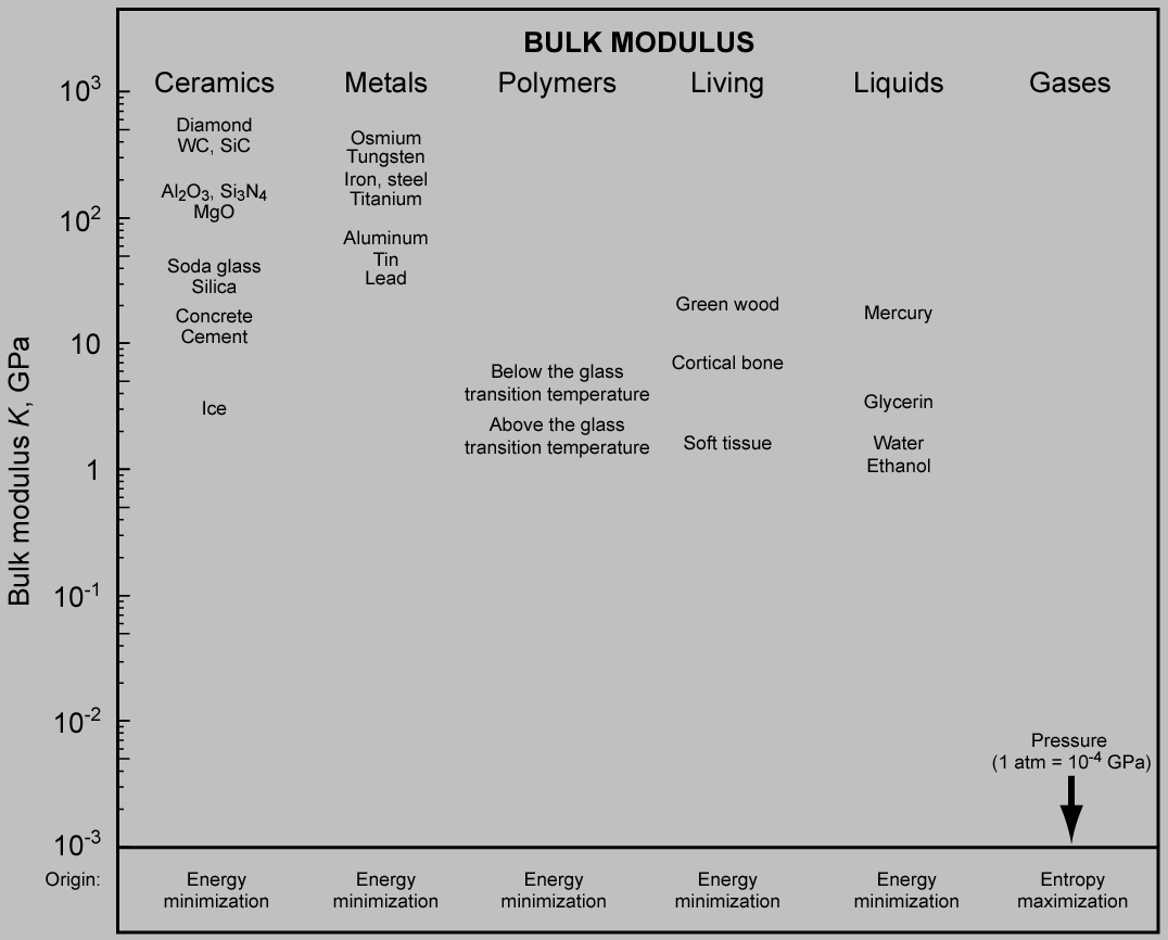
Approximate bulk moduli of a variety of material types and the corresponding origins. For ceramics and solids, the bulk modulus is generally only slightly higher than the shear modulus and retains essentially the same ordering, as mediated by the relation \(K=\frac{2G(1+\nu)}{3(1-2\nu)}\). A more startling transition comes about with the other material classes: the bulk stiffnesses of polymers, biological tissue, and liquids largely converge around 1–10 GPa, and gases assume a finite stiffness that’s roughly equal to their pressure. The stiffness of condensed matter is driven primarily by energy minimization, whereas that of gases is driven primarily by entropy maximization.

The bulk modulus is amazing! It’s got its own neat properties:

• The bulk modulus couples a dilatational load (such as pressure) to a volume change. All stable materials can support hydrostatic pressure, and solids and liquids support such loading easily, with very little deformation, whereas gases dramatically contract or expand. In fact, the bulk modulus across condensed matter doesn’t vary by all that much—a few orders of magnitude, corresponding to the particular strength of the cohesive bonds (covalent, ionic, or metallic, for example). In contrast, the bulk modulus of gases is primarily of entropic origin, the ideal gas featuring no such electrostatic interactions.

  As a result, it works as a first pass to assume that solids and liquids have very high bulk moduli (ten thousand to ten million atmospheres, say), whereas gases have very low bulk moduli that essentially equal their pressure at the time.

• Every stable material compresses under pressure, but pressure can’t destroy a uniform material. In other words, we can apply a very large amount of pressure to a material sample and—barring a temperature increase leading to combustion, for example, or a pressure-induced phase transformation, or transformation into a neutron star or some other exotic effect—we’ll never see anything other than harmless compression. This is why a fragile glass or metal object can fall to the ocean floor and remain unharmed. Recovery expeditions from the RMS Titanic established that even the most fragile solid detritus from the Titanic was structurally undamaged by a pressure of 6000 psi (400 atm):

  
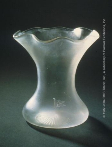
  Selection of fragile glass and ductile metal objects recovered from the RMS Titanic debris field between 1987 and 1994 with no pressure-induced structural damage (http://www.premierexhibitions.com).

• Consider another example: Submarine hulls don’t fail because any specific material element is subjected to hydrostatic pressure. After all, a depth of 2000 m (well beyond the working depth of submarines) would cause a cubic centimeter of steel to compress by only 0.5 μm on a side. Ultimately, submarines driven past their critical depth fail because their hull material isn’t subjected to hydrostatic pressure: the in-hull longitudinal and hoop stresses are far larger than the external pressure (and even larger than the internal pressure), and these differences produce a deviatoric stress state that induces failure.

  Consider the reverse example: a pipe that failed from excessive internal pressure:

  
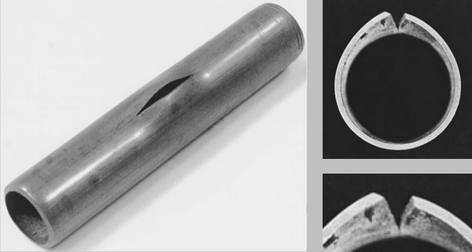
  Failure surfaces of an overpressurized pipe that burst from excessive hoop stress (adapted from photographs by R. A. Simonds, from Courtney’s Mechanics of Materials). The failure mode of this ductile material is shear related, of course, as clearly indicated by the ~45° failure surface.

  Notably, even though this failure ultimately arose from pressure, the failure mode was that of deviatoric stress, as indicated by the near-45° angle in the failure surface—the hallmark of shear.

• The bulk modulus is a great way to start exploring the origins of the elastic moduli in condensed matter and gases. (This section gets a little math intensive.) Very broadly, the (isothermal) bulk modulus \(K\) is defined as the pressure \(P\) needed to achieve a certain decrease in volume per unit volume \(V\) at constant temperature \(T\)—succinctly, \(K\equiv -V(\partial P/\partial V)_{T}\). Let’s also pull in the fundamental thermodynamic equation for a closed system

  $$dU=T\,dS-P\,dV,$$

  which tells us, for example, that we can increase a system’s energy \(U\) either by heating it (i.e., transferring entropy \(S\) to it at a certain temperature \(T\)) or by doing work on it (here, by compressing it, i.e., transferring volume \(V\) away from it at a certain pressure \(P\)). To clarify the influence on \(K\), we isolate \(P\) and perform the necessary differentiation step with respect to volume to obtain

  $$K\equiv-V\left(\frac{\partial P}{\partial V}\right)_T=V\left[\left(\frac{\partial ^2 U}{\partial V^2}\right)_T-T\left(\frac{\partial^2 S}{\partial V^2}\right)_T\right].$$

  In condensed matter, with its strong intermolecular bonds, the energy term containing \(U\) dominates, and so we find that the bulk modulus scales with the curvature of the bond energy as a function of molecular spacing. (Just as the first spatial derivative gives the slope of any function, the second spatial derivative gives the curvature.) This curvature grows more extreme with a deeper—a stronger—bond, and so we observe a correlation between the bulk modulus and the melting temperature, as we can confirm from a trip to Wolfram Alpha:

  
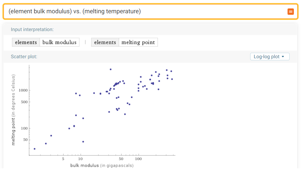
  Stiffer elements tend to be more refractory; both properties depend on the bond strength. (We see a similar trend in the density.)

  Scientists have spent about a century developing pair potential functions to describe the energy \(U\) associated with atoms in close vicinity. These functions describe the tradeoff between the tendency of atoms and molecules to attract when they’re far apart but to repel when they’re close together. With a potential function in hand, predicting the stiffness of adjacent atoms—and by extension, the bulk modulus of the overall material—using the above equation is in theory straightforward by differentiating twice.

  In gases, in contrast, strong intermolecular bonds are absent, and the entropy term containing \(S\) dominates. (Gases have an enormous entropy because of the huge number of positions and velocities that a molecule can explore in the gaseous state.) We can simply insert the equation of state for an ideal gas, \(P=nRT/V\), into the above definition of \(K\) to find that the isothermal bulk modulus for an ideal gas at a certain temperature is exactly \(P\).

Given all this, why not love the bulk modulus?

Mathematical framework

All of the concepts discussed in this note can be summarized in one unified mathematical expression—if you’re into that kind of thing.

It’s called generalized Hooke’s Law, discussed at a slightly more technical level here. That note derives the relationships connecting Young’s modulus, the shear modulus, the bulk modulus, and Poisson’s ratio. But even in that note, I consistently expressed generalized Hooke’s Law in terms of Young’s elastic modulus! What a hypocrite. Here, let’s re-derive generalized Hooke’s Law (for a uniform isotropic material) using those fundamental parameters, the shear and bulk elastic moduli. After all, as shown by the rotated-element example above, all these moduli—and Poisson’s ratio—are intrinsically connected.

OK, so we already know that the shear modulus \(G\) couples the angular shear strain (this turns out to be \(2\epsilon_{xy}\), as discussed in the other note) to the shear stress \(\sigma_{xy}\). Replacing the \(x\), \(y\), \(z\) coordinate system with a 1, 2, 3 coordinate system, we obtain the equations

$$\epsilon_{12}=\frac{\sigma_{12}}{2G};$$

$$\epsilon_{13}=\frac{\sigma_{13}}{2G};$$

$$\epsilon_{23}=\frac{\sigma_{23}}{2G}.$$

We also know that the bulk modulus \(K\) couples the volumetric strain (which is \(\epsilon_1+\epsilon_2+\epsilon_3\) for small strains, as discussed in the other note) with the dilatational stress or negative pressure \((\sigma_{11}+\sigma_{22}+\sigma_{33})/3=-P\):

$$\epsilon_{11}+\epsilon_{22}+\epsilon_{33}=\frac{(\sigma_{11}+\sigma_{22}+\sigma_{33})}{3K}.$$

We can combine all six equations (in a hand-wavy way) into an elegant single equation with the aid of some handy notation:

• An index such as \(i\) or \(j\) can range from 1 to 3 independently.

• A repeated index in a term indicates summation (e.g., \(\sigma_{kk}\) is shorthand for \(\sigma_{11}+\sigma_{22}+\sigma_{33}\)).

• The Kronecker delta \(\delta_{ij}\) is 1 when \(i=j\) and 0 otherwise.

Thus, we have

$$\epsilon_{ij}=\frac{\sigma_{ij}}{2G}-\left(\frac{1}{6G}-\frac{1}{9K}\right)\sigma_{kk}\delta_{ij}.$$

This equation expands into six (!) independent equations that can be used to calculate the normal stresses \(\sigma_{11}\), \(\sigma_{22}\), and \(\sigma_{33}\) and the shear stresses \(\sigma_{12}\), \(\sigma_{13}\), and \(\sigma_{23}\). Note how the \(\frac{1}{6G}\) term on the right negates the \(\frac{1}{2G}\) coefficient of \(\sigma_{ij}\) under the hydrostatic case of \(\sigma_{ii}\delta_{ij}=\sigma_{11}+\sigma_{22}+\sigma_{33}=-3P\). So now we have another version of generalized Hooke’s Law, one that displays the usefulness of elastic moduli other than Young’s modulus.

For maximum utility, though, I want to show generalized Hooke’s Law in four forms—for strains \(\epsilon\) in terms of stresses \(\sigma\) and stresses in terms of strains, using (1) the shear modulus \(G\) and bulk modulus \(K\) and (2) Young’s modulus \(E\) and Poisson’s ratio \(\nu\):

$$\epsilon_{ij}=\frac{\sigma_{ij}}{2G}-\left(\frac{1}{6G}-\frac{1}{9K}\right)\sigma_{kk}\delta_{ij}.$$

$$\epsilon_{ij}=\frac{1+\nu}{E}\sigma_{ij}-\frac{\nu}{E}\sigma_{kk}\delta_{ij}.$$

$$\sigma_{ij}=2G\epsilon_{ij}+\left(K-\frac{2}{3}G\right)\epsilon_{kk}\delta_{ij}.$$

$$\sigma_{ij}=\frac{E}{1+\nu}\epsilon_{ij}+\frac{\nu E}{(1+\nu)(1-2\nu)}\epsilon_{kk}\delta_{ij}.$$

Various other combinations of the elastic moduli and Poisson’s ratio are possible; the individual moduli are coupled by \(E=2G(1+\nu)\) and \(E=3K(1-2\nu)\). All of the equations above tell us the exact same thing, and all might be useful in various scenarios. For example, if we limit ourselves to shear stress and strain, then we can discard the second term on the right-hand side because \(\delta_{ij}=0\). And if we’re in a plane-stress or plane-strain situation in which \(\sigma_{33}=0\) or \(\epsilon_{33}=0\), respectively, then we obtain other useful simplifications. We find, for example, that although the bending stiffness of a beam scales with \(E\), the bending stiffness of a plate scales with \(E/(1-\nu^2)\)—in other words, a plate is effectively stiffer because its width doesn’t allow it to easily deform laterally in the manner of a narrow rod.

But remember that these equations apply only to isotropic* materials deforming linearly and elastically.

A plethora of other elastic moduli

Beyond the shear modulus and bulk modulus (which are certainly appealing for characterizing the steady-state linear elasticity of uniform matter), let’s revel in the many other elastic moduli that practitioners have found useful:

• Certain modifications of Young’s modulus, such as the biaxial modulus \(E/(1-\nu)\) and the plane-strain modulus \(E/(1-\nu^2)\) are used in cases other than a uniaxial stress state, as discussed in the other note. The so-called reduced modulus \([(1-\nu_I^2)/E_I+(1-\nu_S^2)/E_S]^{-1}\), used in indentation studies, effectively combines the plane-strain stiffnesses of an indenter material \(I\) and a substrate material \(S\).

• Various poroelastic moduli apply in the context of materials containing fluid-filled pores—a two-phase system that’s exquisitely sensitive to whether the fluid can drain out of the material into the surrounding environment. These moduli find frequent use by soil scientists, biological tissue engineers, and anyone working with foams or other cellular structures.

• The secant and tangent moduli: For materials such as elastomers that can elastically deform to several times their length (in contrast to metals and ceramics, which generally can’t deform by more than a fraction of a percent without plastically deforming or fracturing), we encounter a strongly nonlinear elastic stress-strain diagram that presents us with a challenge of whether to look at finite or infinitesimal slopes. There’s an elastic modulus for each option.

• Anisotropic elastic moduli emerge when we move from randomly polycrystalline and amorphous materials to polycrystalline materials with a texture—meaning a prevailing orientation—and single-crystal materials, for example. In this case, generalized Hooke’s Law no longer holds, as different elastic moduli might apply in different orientations. In the most extreme example of crystal anisotropy (namely, the triclinic crystal structure with unequal side lengths and angles and arbitrary orientation), 21 (!) independent moduli are needed in theory to describe the material’s static elastic behavior alone.

• Geologists define S-wave and P-wave moduli that are coupled to the speeds of seismic events in a bulk material. The former corresponds simply to the shear modulus; the latter is \(\frac{E(1-\nu)}{(1+\nu)(1-2\nu)}\), which represents the stress needed to obtain a unit strain in a uniaxial strain configuration. (Try verifying this from generalized Hooke’s Law above.)

• Continuing the dynamic theme, instantaneous and equilibrium moduli are used to characterize material deformation over short and long time periods, respectively, for systems where relaxation processes are relevant. (In the very long run, though, every material, including solids, has an equilibrium stiffness of zero. In the words of Prof. Chris Schuh at MIT, there’s no such thing as elasticity; there’s only negligible plasticity. At any temperature, materials creep, or deform over time, under any finite load. One notable example is lead pipes sagging over decades. But the stories of window glass sagging over human-relevant timespans are myths. The covalent bonds in silica glass are sufficiently strong that it would take aeons to notice gravity-driven creep at room temperature.)

• The complex modulus \(G^\prime(\omega)+iG^{\prime\prime}(\omega)\) quantifies the dynamic stiffness as a function of an oscillation frequency \(\omega\). The \(G^\prime\) component alone corresponds to the shear stiffness \(G\) of an ideal solid, whereas \(G^{\prime\prime}\) alone corresponds to the strain-dependent stiffness of an ideal liquid (whose stiffness generally scales up with the strain rate, as mediated by the viscosity). Their combination provides the so-called viscoelastic response. The imaginary unit \(i\) indicates that the deformation of a liquid lags behind that of a solid. That lag arises because if you shear and release a solid, it springs back; if you shear and release a liquid, it deforms and sits, and you’d have to pull it back to restore the original configuration.

With this information in mind, the next time you hear about an “elastic modulus,” consider: are they talking about Young’s elastic modulus or another elastic modulus? And are they using the appropriate framework to analyze and present their results? Again, let’s not overrate Young’s modulus; instead, let’s appreciate its advantages while understanding its limitations and what insights come with a familiarity with other types of stiffness.