The electrothermal model introduced in Chapter 3 employs a linear differential equation, written as Equation (4), to represent the temperature of a suspended beam undergoing resistive heating. Thermal expansion is calculated in Equation (9) by integrating the expansion of a differential element. It was found that the thermal conductivity ks and the thermal expansion coefficient a of silicon cannot be considered to be independent of temperature, due to the large temperature range over which the actuators operate. Consequently, the heat and thermal expansion equations become nonlinear. However, the temperature distribution can be solved numerically by using approximate equations, in which derivatives are approximated by finite differences and integrals by finite summations [51].
Because the temperature distribution in a V-beam actuator is symmetric, only half of the beam is considered. The boundary conditions consist of a fixed temperature T¥ where the beam is attached to the anchor and an adiabatic condition at the midpoint of the beam, representing the symmetry of the temperature distribution. By dividing the left half of the beam into N nodes, Equation (4) and (9) are rewritten as
By using Equations (41) and (42), the values of the temperature-dependent properties can be calculated at each node. Additionally, the temperature distribution can be calculated by solving Equation (50). The solution is found by alternating between these two steps in an iterative process until the temperature distribution has converged to a sufficient degree.
The following program has been written in MATLAB to solve for the temperature distribution and the midpoint deflection of V-beam actuators.
clear all
%
% Input beam properties
%
Laa=1000e-6;
g=2e-6;
h=50e-6;
d=10e-6;
L=2*sqrt((Laa/2)^2+d^2);
%
% Material properties
%
rho=0.000133;
ka=0.026;
(15) E=166e9;
Tinf=298;
%
% Calculate w', S, A, I
%
R=266;
w=rho*L/h/R;
S=4/w*(1e-6+g)+1;
A=w*h;
I=w^3*h/12;
%
% Assemble matrices
%
i=.03;
J=i/w/h;
N=10;
dx=L/N/2;
for j=1:N-1
B(j,j+1)=-1;
B(j+1,j)=-1;
T=ones(N,1)*Tinf;
Told=zeros(N,1);
%
% Iteration subroutine
%
while abs(max(T-Told))>1e-3
Told=T;
ks=exp(-1.28*log(Told)+12.28);
C=C+eye(N)*S*ka/g/h;
D=S*ka*repmat(Tinf,N,1)/g/h+J^2.*rho;
end
%
% Calculate average temp and thermal strain
%
max_temp=max(T)
for j=1:N-1
G(j+1,j)=1;
end
Tel=G*T/2;
ave_temp=mean(Tel)
alpha=(3.725*(1-exp(-5.88e-3*(Tel-124)))+5.548e-4*Tel)*1e-6;
%
% Calculate flexibility matrix and deflection
%
F(1,1)=L^3/3/E/I+8*d^2/L/E/A;
F(1,2)=5*L^2*d/12/E/I-2*d/E/A;
F(1,3)=-L^2/2/E/I;
F(2,1)=F(1,2);
F(2,2)=2*L*d^2/3/E/I+L/E/A;
F(2,3)=-L*d/2/E/I;
F(3,1)=F(1,3);
F(3,2)=F(2,3);
F(3,3)=L/E/I;
X=F\[-2*d*del/L del 0]';
u=L^2/48/E/I*(X(1)*L-6*X(3))
The operation of this program is demonstrated by using a beam segment divided into four elements, as shown in Figure 41. To illustrate how the temperature distribution can be found with matrix algebra, Equation (50) is rewritten as
where temperatures are evaluated at the nodes between elements and Ti' represents the temperature distribution used to approximate the thermal conductivity. This distribution is initially assumed to be equal to the ambient temperature and is successively revised as the program converges to a solution.
Figure 41. Element and node locations of V-beam actuator used in numerical solution.
Equation (52) can be rewritten in the following matrix form:
(53)

where
(54)

and
These matrices are constructed in lines (32) through (36) and (46) through (48) of the program. The boundary conditions are enforced in lines (37) and (49) by doubling the value of the C43 coefficient to represent the adiabatic condition and by including the second term in Equation (55), which represents the fixed temperature at the anchor.
The nodal temperature distribution T is calculated in line (50) by using matrix inversion. The thermal conductivity is then recalculated using the values in T (now Ti'), and the loop repeats. Iteration continues until the maximum difference between successive nodal temperature distributions is smaller than a chosen error value.
The elemental temperature distribution is calculated in lines (56) through (61) by using the following equation:
(56)

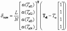
The thermal expansion of the entire actuator is calculated in line (64) as
(57)

and the deflection at the midpoint is calculated using the flexibility method introduced in the thermomechanical analysis in Chapter 3.
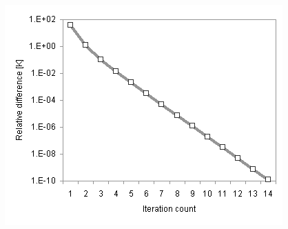
Because each of the two temperature-dependent variables tends to increase deflection at higher temperatures, the program is expected to yield a unique solution. The speed of convergence of the program is demonstrated in Figure 42.
Figure 42. Convergence of numerical solution for electrothermal analysis.


